STATISTICS with R
McNemar’s Test in R
McNemar’s test is a nonparametric statistical method applied to paired or related dichotomous variables, designed to assess whether the proportion of binary outcomes changes significantly between two related measurements. It is particularly useful in before‑and‑after study designs, where the objective is to determine if an intervention, treatment, or exposure has produced a meaningful shift or flip in participants’ responses.
Introduction to McNemar’s Test
When comparing two related measurements, the paired samples t-test is typically employed to assess mean differences for paired continuous variables. However, in many applied research settings—such as program evaluations and pre‑post intervention studies—data are frequently collected as dichotomous or binary responses rather than continuous measurements. When the outcome variable represents categories such as “yes/no,” “correct/incorrect,” or “support/oppose,” the t-test is no longer suitable. In these situations, McNemar’s test is the appropriate statistical procedure, as it determines whether the proportion of individuals within a given category changes between two time points. In addition, because the measurements are related, a chi-squared test of independence should not be used, either.
McNemar’s test is based on a 2×2 contingency table that cross‑tabulates each participant’s responses at Time 1 and Time 2. The diagonal cells, referred to as concordant pairs, indicate individuals whose responses remained unchanged across both time points and are excluded from the calculation of the test statistic. The analysis centers solely on the discordant pairs, representing participants whose responses shifted between measurements. McNemar’s test statistic evaluates whether there is a statistically significant difference between the counts of “yes → no” transitions and “no → yes” transitions. A significant imbalance between these two categories of discordant pairs may indicate that the intervention or condition had an impact on the distribution of responses.
McNemar’s test is suitable when the same individuals provide dichotomous responses at two distinct time points or occasions. Common applications include public health interventions (such as assessing willingness to receive a vaccination before and after an informational session), diagnostic comparisons (such as contrasting positive or negative results from two screening tools applied to the same patients), and instructional evaluations (such as measuring correct versus incorrect responses before and after a brief tutorial). In all instances, the objective is to determine whether the proportion of individuals in a given category has shifted in a statistically significant manner.
The data collected to perform the McNemar’s test could be in the form of raw data (Table 1) or in a summary table called a crosstab or contingency table (Table 2).
| Resident | Support (Before) | Support (After) |
|---|---|---|
| Resident 1 | Support | Support |
| Resident 2 | Support | Do Not Support |
| Resident 3 | Do Not Support | Support |
| Resident 4 | Support | Support |
| Resident 5 | Do Not Support | Do Not Support |
| … | … | … |
A crosstab or contingency table presents the sum of the counts from a raw data table.
| Opinion (Before) | Do Not Support (After) | Support (After) |
|---|---|---|
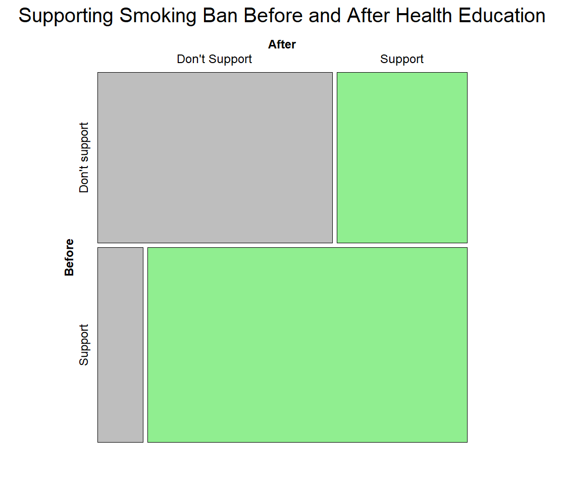
| Do Not Support | 45 | 25 |
| Support | 10 | 70 |
In the following sections, we present an example scenario where the McNemar’s test will be used to analyze the data using base R code and functions.
McNemar’s Test Example
Is there a change in a condominium residents’ support for banning smoking within 25 feet of building entrances after a health‑education program?

Residents of a large condominium complex participated in a survey to determine their stance on prohibiting smoking within 25 feet of all building entrances. Initially, the building association distributed the questionnaire to establish baseline opinions prior to any outreach. Subsequently, it implemented a concise health‑education initiative comprising informational materials and brief presentations highlighting how smoke‑free entryways can reduce exposure to secondhand smoke, enhance air quality, and foster a healthier shared environment. Following this program, the same residents completed the questionnaire again. As each individual provided paired, dichotomous responses (support versus do not support), the resulting before‑and‑after data present an ideal scenario for applying McNemar’s test, which assesses whether the health‑education intervention led to a statistically significant change in residents’ support for the proposed smoking‑ban policy.
| Resident | Support (Before) | Support (After) |
|---|---|---|
| Resident 1 | Support | Support |
| Resident 2 | Support | Do Not Support |
| Resident 3 | Do Not Support | Support |
| Resident 4 | Support | Support |
| Resident 5 | Do Not Support | Do Not Support |
| … | … | … |
The complete data set for this example can be downloaded from here.
Analysis: McNemar’s Test in R
The McNemar test is a statistical method used to assess changes in paired categorical responses, particularly when each participant provides a dichotomous (yes/no, correct/incorrect) answer at two distinct time points. Rather than analyzing relationships between two independent categorical variables, it focuses on before‑and‑after data from the same individuals. In this example, the aim is to determine whether the health education program was effective by examining changes in opinions about banning smoking using McNemar’s test. Listing 1 includes the R code to run McNemar’s test on our data.
# Read the data
dfOpinonSmoking <- read.csv("df_opinion_smoking_ban.csv")

# Create contingency / crosstab table
tbOpinion <- table(dfOpinonSmoking$opinion_before, dfOpinonSmoking$opinion_after)

# Print out contingency table
print(tbOpinion)

# Run McNemar's test
mcnemar.test(tbOpinion)

# Output

               dont_support support
  dont_support           45      25
  support                10      70


	McNemar's Chi-squared test with continuity correction

data:  tbOpinion
McNemar's chi-squared = 5.6, df = 1, p-value = 0.01796The R code in Listing 1 shows that first convert the raw count data into a contingency table and then input the contingency table into the mcnemar.test() function, which is built-in R function (we do not need to install and call a package).
The contingency table presents the distribution of supporting and opposing responses recorded before and after the implementation of the health‑education program (Figure 1). Results from McNemar’s test indicate a statistically significant change, with . Given that most of the new responses reflect support for prohibiting tobacco use near building premises, it can be concluded that the health‑education program achieved its intended effect.