STATISTICS with R
ANCOVA in R
ANCOVA (analysis of covariance) is a commonly used statistical technique for comparing the mean values of multiple groups on a continuous outcome while accounting for the influence of a related continuous variable. It extends ANOVA (analysis of variance) by incorporating a continuous independent variable into the model to reduce bias and control for potential confounding effects from that variable, known as the covariate or controlling variable. ANCOVA can be conducted within both the ANOVA framework and the linear modeling framework, such as multiple regression.
Introduction to ANCOVA
When comparing the means of two or more groups, various statistical methods can be applied, such as t-tests, ANOVA, or regression models. For instance, a researcher examining the effects of two medications on blood pressure might use a t-test to determine whether the mean differences between the treatment groups are statistically and clinically significant. However, these differences could partly result from other factors, such as participants’ initial blood pressure, BMI, or other confounding variables, potentially biasing the results.
A common approach to reducing bias and within-group error variance in observational or quasi-experimental data is to incorporate control variables (covariates) that are believed to influence the outcome. In other words, independent variables beyond the primary factors in the experiment or study may be correlated with the outcome of interest (e.g., the treatment effect). In such cases, statistical techniques like analysis of covariance (ANCOVA) can be employed to adjust outcome measurements for the presence of influential covariates. Adjusting for a covariate may alter the observed outcome values.
ANCOVA is an extension of ANOVA that incorporates an additional continuous covariate believed to confound the relationship between research variables. Like ANOVA, ANCOVA results allow for the comparison of means across two or more groups after adjusting for the confounding variable. In essence, it removes variance attributable to the covariate as well as within-group error variance. When an ANCOVA test yields statistical significance, post hoc or contrast tests (such as Bonferroni) can be conducted to determine which group means differ significantly after controlling for the covariates.
Like an ANOVA test, an ANCOVA test also comes with certain assumptions that need to be met, such as,
- Linearity — The covariate must have a linear relationship with the dependent variable.
- Homogeneity of regression slopes — The covariate–outcome relationship must be the same across all groups (tested via the group × covariate interaction).
- Independence of the covariate and treatment — The covariate must be measured before treatment and must not be affected by it.
- Normality and homoscedasticity of residuals — Standard linear model assumptions apply.
Before conducting ANCOVA, it is essential to verify the assumption of homogeneity of regression slopes, ensuring no significant interaction between the group and the covariate. The following sections present an example research scenario using ANCOVA to analyze the data.
ANCOVA Example
Is there a difference in jump performance between female and male high jump athletes, and does this difference persist after accounting for the athletes’ heights?

A sports scientist wants to find out if male and female high jumpers differ in their performance, and whether those differences still exist after considering the athletes’ height.
High jump performance is influenced by biomechanical and physiological factors, including strength, technique, and body structure. Height can offer a mechanical advantage in these events, and male athletes are, on average, taller than female athletes. Consequently, observed gender differences in performance may be partly attributed to variations in height rather than gender alone.
The sports scientist decides to verify this hypothesis using data collected from female and male athletes from a high school. The researcher collects data on how high the athletes have jumped (in centimeters), their gender (female, male), and their heights (in centimeters). Table 1 shows the data for five athletes.
| Sex | Height (cm) | Jump (cm) |
|---|---|---|
| Female | 161.6 | 108.5 |
| Female | 163.6 | 134.3 |
| Male | 176.5 | 126.9 |
| Male | 170.8 | 121.7 |
| Female | 174.4 | 136.7 |
| … | … | … |
In this study, the sports scientist aims to determine whether female and male athletes differ in their jump performance. Furthermore, the researcher seeks to assess whether accounting for the athletes’ heights would influence the observed results. After collecting the data and verifying the necessary assumptions, the researcher conducts a one-way analysis of variance (ANOVA) to compare jump performance between genders. To control for athletes’ heights, an analysis of covariance (ANCOVA) is performed, including height as a covariate. The dataset for this example is available for download in CSV format.
Analysis: ANCOVA in R
In this study, the sports scientist aimed to determine whether female and male athletes differ in high jump performance. Alongside data on performance and sex, the scientist collected information on athletes’ heights to assess whether any performance differences could be attributed to height. The researcher first calculates the descriptive statistics of the unadjusted jump heights for female and male athletes. Next, the sport scientist runs an ANOVA to compare high jump performance between female and male athletes, followed by an ANCOVA incorporating height as a covariate. While an independent samples t-test could be used for two groups, ANOVA was chosen to facilitate comparison with ANCOVA. Listing 1 shows the R code for descriptive statistics and ANOVA testing.
# ANCOVA in R
# Load required packages
library(car) # Type III SS
library(emmeans) # Estimated marginal means
library(dplyr)

# Read in data
dfHighJump <- read.csv("df_high_jump_hurdle.csv")

# Descriptive statistics
dfHighJump %>%
  group_by(sex) %>%
  summarise(
    mean_jump = mean(highjump_cm, na.rm = TRUE),
    sd_jump   = sd(highjump_cm, na.rm = TRUE),
    n         = n()
  )

# Perform ANOVA (sex as the factor)
options(contrasts = c("contr.sum", "contr.poly"))
fitAnova <- aov(highjump_cm ~ sex, data = dfHighJump)
Anova(fitAnova, type = 3)
TukeyHSD(fitAnova, 'sex')

# Output 1: descriptive statistics
# A tibble: 2 × 4
  sex    mean_jump sd_jump     n
  <chr>      <dbl>   <dbl> <int>
1 female      122    9.10    21
2 male        135    8.03    21


# Output 2: ANOVA table
Anova Table (Type III tests)

Response: highjump_cm
            Sum Sq Df  F value    Pr(>F)
(Intercept) 310226  1 4213.051 < 2.2e-16 ***
sex           1801  1   24.453 1.411e-05 ***
Residuals     2945 40
---
Signif. codes:  0 ‘***’ 0.001 ‘**’ 0.01 ‘*’ 0.05 ‘.’ 0.1 ‘ ’ 1

# Output 3: Tukey HSD pairwise test
  Tukey multiple comparisons of means
    95% family-wise confidence level

Fit: aov(formula = highjump_cm ~ sex, data = dfHighJump)

$sex
                diff      lwr      upr    p adj
male-female 13.09524 7.743084 18.44739 1.41e-05
In Listing 1 above, the sports scientist computes the mean jump heights for female and male athletes, which are 122 cm and 135 cm, respectively. These are the unadjusted means. Apparently, on average male athletes jump higher. An ANOVA test also shows that the sex factor is statistically significant (p < 0.05). A follow-up pairwise comparison using Tukey HSD familywise error correction also shows the mean difference between male and female athletes is statistically significant.
However, the sports scientist decides to include the heights of the athletes as a covariate because based on previous research, height could be correlated with how high the athletes jump. Therefore, the sports scientist conducts an ANCOVA to compare adjusted means between female and male athletes. Listing 2 shows the R code to run ANCOVA.
# Test interaction assumption
fitInteraction <- aov(highjump_cm ~ sex * height_cm, data = dfHighJump)
Anova(fitInteraction, type = 3)

# Perform ANCOVA (sex as factor and height as covariate)
fitANCOVA <- aov(highjump_cm ~ sex + height_cm, data = dfHighJump)
Anova(fitANCOVA, type = 3)

# Output 1: ANOVA with interaction table
Anova Table (Type III tests)

Response: highjump_cm
               Sum Sq Df F value    Pr(>F)
(Intercept)     95.11  1  2.1207    0.1535
sex             32.17  1  0.7174    0.4023
height_cm      849.87  1 18.9489 9.776e-05 ***
sex:height_cm   30.63  1  0.6829    0.4137
Residuals     1704.32 38
---
Signif. codes:  0 ‘***’ 0.001 ‘**’ 0.01 ‘*’ 0.05 ‘.’ 0.1 ‘ ’ 1


# Output 2: ANCOVA table
Anova Table (Type III tests)

Response: highjump_cm
             Sum Sq Df F value    Pr(>F)
(Intercept)   66.91  1  1.5042    0.2274
sex            9.04  1  0.2031    0.6547
height_cm   1210.43  1 27.2093 6.316e-06 ***
Residuals   1734.95 39
---
Signif. codes:  0 ‘***’ 0.001 ‘**’ 0.01 ‘*’ 0.05 ‘.’ 0.1 ‘ ’ 1
In Listing 2, the sports researcher first runs an ANOVA with interaction term between sex and height to assess the assumption of no interaction between factor and covariate. The results in output 1 show that the interaction between sex and height is not statistically significant. Therefore, the sports scientist runs an ANCOVA.
According to the ANOVA results (output 2), after entering height as a covariate, the sex factor is no longer statistically significant (p = 0.65). This contradicts the ANOVA results, where sex was a significant factor. The covariate explains additional variance in jump height, reducing residual error and removing the apparent group difference. Therefore, the sports scientist can conclude that after adjusting for the heights of the athletes, no significant difference was found between female and male athletes in their performance in high jump sport.
How did the inclusion of height as a covariate change the means in each sex? The mean values after adjusting for a covariate are called marginal means (or conditional means). Listing 3 shows the R code to compute marginal means for female and male athletes and pairwise comparison of the means using Tukey HSD adjustment.
# Jump means per sex adjusted for heights
emm <- emmeans(fitANCOVA, ~ sex)

# View adjusted means
emm

# Pairwise comparisons
pairs(emm, adjust = "tukey")

# Output 1: marginal means
sex    emmean   SE df lower.CL upper.CL
 female    127 1.84 39      124      131
 male      129 1.84 39      125      132

# Output 2: Pairwise comparions
contrast      estimate   SE df t.ratio p.value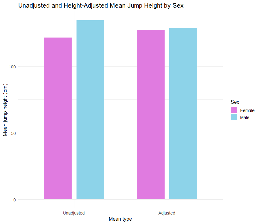
female - male -1.37 3.05 39 -0.451 0.6547In Listing 3, we can see that after adjusting for heights, the mean jumps for female and male athletes are very close to each other (output 1). On average female athletes scored 127 cm and male athletes scored 129 cm. The pairwise comparison (output 2), shows that the mean difference is not statistically significant (p = 0.654). These results also confirm that after controlling for height, there is no statistically significant difference between female and male athletes in high jump sport. Figure 1 compares the mean jump values before and after adjusting for athletes’ heights.
Reporting ANCOVA Results
A sports scientist investigated whether male and female high‑jump athletes differ in performance and whether any disparity persists after controlling for height. Using data on athletes’ sex, height, and jump height, the researcher first conducted a one‑way ANOVA, revealing that males appeared to outperform females. An ANCOVA was then performed with height as a covariate. After adjusting for height, the effect of sex was no longer statistically significant (p = .655), and the adjusted means for males and females were nearly identical, indicating that the initial difference was primarily attributable to height rather than sex.