STATISTICS with R
A comprehensive guide to statistical analysis in R
Two-way ANOVA in R
Two-way ANOVA, or two-way analysis of variance, is a statistical method used to compare the mean values of a continuous dependent variable across groups defined by two categorical independent variables (also called factors). A two-way ANOVA test not only evaluates the main effects of each factor on the dependent variable but also determines whether there is an interaction effect between the two factors, and if simple effects are statistically significant. Like the one-way ANOVA, post hoc tests can be performed following a significant result to identify specific group differences (main effects, interaction effects, and simple effects).
Introduction to Two-way ANOVA
Two-way ANOVA is a statistical method used when researchers want to compare average values across groups defined by two categorical variables (factors). For instance, a study might explore how education level (high school or lower, bachelor’s degree, graduate degree) and work experience (novice, experienced) work together to influence income. In this case, education level and work experience are the categorical independent variables, while income is the continuous dependent variable. Because there are two factors in this example, we can analyze the data using a two-way ANOVA.
In ANOVA, an independent variable is called a factor, which is a categorical variable with two or more categories or levels. For example, educational attainment could be a factor with three levels: high school or lower, bachelor’s degree, and graduate degree, while work experience might have levels like novice and experienced. Since ANOVA is used to examine factors and their levels, experiments using it are known as factorial designs. When a study includes two factors, it’s called a two-way ANOVA, which looks at the interactions between multiple independent variables. ANOVA with several factors may be called n-way ANOVA.
The main goal of running a two-way ANOVA is to see not just if each factor has a significant impact on the dependent variable (the main effects), but also if there’s a significant interaction between the factors. An interaction happens when the effect of one factor changes depending on the level of another. If the factors as a whole are statistically significant, pairwise comparisons can be done to pinpoint specific group differences. If neither the factors nor their interaction are significant, the analysis usually stops at that point.
In the next sections, we’ll walk through an example research scenario using a two-way ANOVA to analyze the data. We’ll show you step-by-step how to run the test in R and explain how to interpret the results.
Two-way ANOVA Example
Does the type of physical therapy affect the recovery time of patients after knee surgery? And does the recovery time depend on the severity of the knee surgery?
A health researcher conducts a study to investigate whether different types of physical therapy and the severity of knee injuries influence the recovery time of patients after undergoing knee surgery. The study includes three groups of patients based on the type of physical therapy:
- Group 1: Patients receiving no physical therapy (Control)
- Group 2: Patients receiving Standard physical therapy (Standard)
- Group 3: Patients receiving Advanced physical therapy (Advanced)
Patients are further categorized based on the severity of their knee injuries: Moderate or Severe. This creates a total of six subgroups (e.g., Moderate severity patients receiving Standard Physical Therapy, Severe severity patients receiving Standard Physical Therapy, etc.). After the surgery, the researcher records the number of days it takes for each patient to fully recover. Recovery time is measured in days. Patients are randomly recruited from different sites and randomly assigned to both physical therapy groups and severity subgroups to ensure balanced representation.
In this study design, there are two factors: (1) physical therapy method, with three categories (Standard physical therapy, Advanced physical therapy, No physical therapy or the Control group), and (2) knee injury severity, with two categories (Moderate, Severe). The dependent variable, recovery time measured in days, is continuous. Therefore, a two-way ANOVA is appropriate to address the research question. The two-way ANOVA will evaluate the main effects of physical therapy method and injury severity, as well as the interaction effect between these two factors.
In statistical terms, an interaction effect can be considered as a type of moderation when the influence of one independent variable on a dependent variable is affected by a second independent variable. This second variable, known as the moderator, shapes the strength, direction, or nature of the relationship between the primary independent variable and the dependent variable. For example, the effectiveness of a physical therapy method (primary independent variable) on recovery time (dependent variable) may vary depending on the severity of the patient’s injury (moderator). In this case, injury severity “moderates” the relationship between the therapy method and recovery time, indicating that the therapy’s effect is not consistent across all levels of injury severity. Interaction as moderation is commonly analyzed using multiple regression techniques. When the term “moderator” is used for a variable, it is usually assumed that that variable is not the primary variable of interest.
If the ANOVA results reveal significant effects, post hoc tests can be conducted to determine which specific groups or combinations of factors differ significantly. This design allows the researcher to understand both the independent and combined effects of physical therapy method and injury severity on recovery time. Table 1 shows the recovery time in days of six patients in three different physical therapy treatments and two different knee injury severities (moderate, serious).
| Patient | Treatment Group | Severity | Recovery Time (days) |
|---|---|---|---|
| Patient 1 | Control | Moderate | 34 |
| Patient 2 | Control | Severe | 36 |
| Patient 3 | Standard | Severe | 24 |
| Patient 4 | Advanced | Moderate | 28 |
| Patient 5 | Standard | Severe | 23 |
| … | … | … | … |
The researcher is interested in understanding whether physical therapy method and knee injury severity have an effect on the recovery time of patients after knee surgery. Additionally, the researcher aims to determine which therapy method is most effective and how the severity of the injury may moderate these effects. Patients are categorized by physical therapy methods (Standard, Advanced, and Control) and knee injury severity (Moderate, Severe), creating six groups overall. Recovery time is recorded in days when the physical therapist certifies full recovery and the patient feels comfortable walking. The data for this example can be downloaded in the in CSV format.
Analysis: Two-way ANOVA in R
In the first step, we install two required R packages, namely “car” and “emmeans”. We use the “car” package to perform a two-way ANOVA with Type III sum of squares. We use the “emmeans” library to compute (marginal) means and perform post-hoc tests. The reason that we do not use the base R built-in function aov(), as we did for one-way ANOVA, is that we want to specify the type of sum of squares in the model. Type III sum of squares is the most frequently used type because it accounts for imbalanced designs. The following code in Listing 1 shows the formula approach to perform two-way ANOVA in R with an interaction between the two factors (shown by * in the formula notation.)
# Two-way ANOVA with interaction
library(car)
library(emmeans)

dfTherapy <- read.csv("dfPhysicalTherapySeverity.csv", stringsAsFactors = TRUE)

# Fit linear model with sum contrasts
options(contrasts = c("contr.sum", "contr.poly"))
factorialModel <- lm(Recovery_Time ~ Method * Severity, data = dfTherapy)

# Perform Type III ANOVA
Anova(factorialModel , type = 3)

# Output
Anova Table (Type III tests)

Response: Recovery_Time
                Sum Sq Df    F value  Pr(>F)
(Intercept)      46317  1 11319.8746 < 2e-16 ***
Method            4056  2   495.6437 < 2e-16 ***
Severity             6  1     1.5476 0.21769
Method:Severity     29  2     3.5410 0.03436 *
Residuals          282 69
---
Signif. codes:  0 ‘***’ 0.001 ‘**’ 0.01 ‘*’ 0.05 ‘.’ 0.1 ‘ ’ 1
The output of the two-way ANOVA in Listing 1 shows the ANOVA table, which includes the Type III Sum of Square, Degrees of Freedom (DF), the F value, and the probability (statistical significance) for each factor and the interaction between the factors. The factors include the Method, Severity, and their interaction. According to the results, treatment Method factor is statistically significant (. This means that recovery time from injury significantly depends on which treatment method patients had received. Severity of injury, however, is not a statistically significant factor (. In addition, the interaction between Method and Severity is statistically significant (.
Because the interaction between Treatment and Severity factors is statistically significant, we can perform post hoc comparison tests to compare Treatment methods across Severity levels (simple effects.) For this purpose, we use the functions pairs() from the “emmeans” library. However, first we need to know mean recovery times for each Treatment method across Severity levels. Listing 2 provides R code to compute the average recovery times within each Severity level (called marginal means). Listing 2 provides R code for the post hoc comparison test after a statistically significant two-way ANOVA.
# Two-way ANOVA with interaction
library(car)
library(emmeans)

dfTherapy <- read.csv("dfPhysicalTherapySeverity.csv", stringsAsFactors = TRUE)

# Fit linear model with sum contrasts
options(contrasts = c("contr.sum", "contr.poly"))
factorialModel <- lm(Recovery_Time ~ Method * Severity, data = dfTherapy)

# Perform Type III ANOVA
Anova(factorialModel , type = 3)

# Estimated marginal means (simple effects)
modelMethod <- emmeans(factorialModel, ~ Method | Severity)
print(modelMethod)

# Output
Severity = Moderate:
 Method   emmean    SE df lower.CL upper.CL
 Advanced   17.4 0.522 69     16.4     18.4
 Control    34.7 0.640 69     33.4     36.0
 Standard   24.4 0.561 69     23.3     25.5

Severity = Severe:
 Method   emmean    SE df lower.CL upper.CL
 Advanced   15.1 0.640 69     13.8     16.4
 Control    34.5 0.522 69     33.5     35.6
Standard 25.1 0.584 69 23.9 26.2The output in Listing 2 shows the descriptive statistics (mean, standard error of the mean, and lower and upper confidence intervals of the means) for treatment Methods across two severity levels (Severity = Moderate and Severity = Severe). In the Moderate level of Severity, we can see that the mean recovery time is shortest in Advanced treatment method (17.4 days), followed by Standard treatment method (24.4 days) and lastly the Control group (24.4) days. The same order of recovery time can be observed in the Severe level of Severity. Figure 1 shows the mean recovery time for each treatment effect across severity of the injury. So, we can guess that Advanced method is the most effective physical therapy method. But are these differences in mean recovery times statistically significant? We can run pair-comparison tests using the R code in Listing 3 to answer this questions.
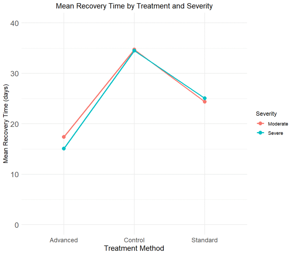
According to the output in Listing 2 and the mean plot in Figure 1, we can guess that Advanced method is the most effective physical therapy method (with the shortest mean recovery time among the treatment groups). But are these differences in mean recovery times statistically significant? We can run pair-comparison tests using the R code in Listing 3 to answer this questions.
# Two-way ANOVA with interaction
library(car)
library(emmeans)

dfTherapy <- read.csv("dfPhysicalTherapySeverity.csv", stringsAsFactors = TRUE)

# Fit linear model with sum contrasts
options(contrasts = c("contr.sum", "contr.poly"))
factorialModel <- lm(Recovery_Time ~ Method * Severity, data = dfTherapy)

# Perform Type III ANOVA
Anova(factorialModel , type = 3)

# Estimated marginal means (simple effects)
modelMethod <- emmeans(factorialModel, ~ Method | Severity)

# Pairwise comparisons
pairs(modelMethod)

# Output
Severity = Moderate:
 contrast            estimate    SE df t.ratio p.value
 Advanced - Control    -17.30 0.826 69 -20.949  <.0001
 Advanced - Standard    -6.98 0.767 69  -9.112  <.0001
 Control - Standard     10.32 0.851 69  12.124  <.0001

Severity = Severe:
 contrast            estimate    SE df t.ratio p.value
 Advanced - Control    -19.43 0.826 69 -23.533  <.0001
 Advanced - Standard    -9.98 0.866 69 -11.527  <.0001
 Control - Standard      9.45 0.783 69  12.062  <.0001

P value adjustment: tukey method for comparing a family of 3 estimates The output in Listing 3 shows two tables for the two levels of Severity (Severity = Moderate and Severity = Severe). In other words, we compare the mean recovery times across treatment Methods once when Severity is moderate and once when Severity is severe (because of significant interaction between Method and Severity). The Tukey adjustment has been applied to control for the family-wise error due to multiple comparison. In each Severity level, three pair-comparisons have been made: Advanced versus Control, Advanced versus Standard, and Control versus Standard. The column estimate shows the difference between the mean recovery times of the two groups being compared. We want to know if such differences between the mean scores of the groups are statistically significant.
The pair-comparisons show that both in Moderate and Severe knee injury levels, the recovery time is statistically significantly different between Advanced, Standard, and Control treatment groups (). As shown in Listing 2, recovery time is shortest in the Advanced treatment group, followed by Standard method, and lastly the Control group.