STATISTICS with R
A comprehensive guide to statistical analysis in R
Pearson Correlation in R
The Pearson (product moment) correlation is a statistical method that measures the linear relationship between two continuous variables (interval or ratio scales variables). The Pearson correlation coefficient value ranges from -1 to 1. Pearson correlation coefficients near -1 or 1 show very high correlation and values close to zero show very weak correlations. A correlation coefficient of zero means there is no correlation between the two variables. The Pearson correlation coefficient (r) is also known as Pearson’s product moment correlation.
Introduction to Pearson Correlation
When there are several random variables in a study or a data set, some of those variables may be related to each other. For example, suppose we collect data on the number of hours participants exercise and the amount of their body fat. Common sense suggests that the more hours participants do exercises, the less body fat they will have. In other words, there is a correlation between the number of hours done exercising and the amount of body fat.
We can quantify this relationship between two variables using a correlation coefficient. The statistical method used to quantify this relationship depends on the nature of the data. If both variables are continuous (or on the interval / ratio scale) and their relationship is linear, we can use Pearson correlation to measure the strength, the direction, and the significance of the correlation.
The strength (or magnitude) of a correlation shows how closely related are the two variables. The strength of a correlation is standardized to fall between -1 and +1. A correlation of 0 means the two variables are totally unrelated (similar to a plus sign, technically called orthogonal). The other characteristic of a correlation is the direction, which is either positive or negative. A positive correlation means that the values of both variables change together: either increasing together or decreasing together. However, if the values of one variable increase while the values of the other variable decrease, the correlation value will have a negative sign. A negative correlation coefficient does not mean a weak relationship; rather, it means the two variables have opposite values. Finally, a correlation could be statistically significant. However, the strength of correlation usually is considered primary. This is because sometimes a very weak correlation coefficient near zero (e.g., 0.03) could still be statistically significant, but not practically significant or meaningful.
In the following sections, we demonstrate an example of a linear relationship between two random variables and provide R code to quantify the strength, direction, and the statistical significance of the linear relationship using Pearson correlation.
Pearson Correlation Example
Is there a relationship between the number of hours students study and their test scores?

A high school teacher is interested in understanding the relationship between the number of hours their students spend studying for a test and the scores the students achieve on the test. The teacher randomly selects 50 students from the school district and asks the students how much time they dedicated to preparing for the test. After collecting the data, the teacher can perform a Pearson correlation test to find out the strength of the relationship, the direction of the correlation, and if the correlation is statistically significant. Table 1 includes the scores of five students on the test.
| Student | Study Hours | Test Score |
|---|---|---|
| Student 1 | 31 | 70 |
| Student 2 | 32 | 75 |
| Student 3 | 44 | 100 |
| Student 4 | 32 | 80 |
| Student 5 | 28 | 83 |
| … |
The teacher enters the data in a spreadsheet program in the school computer lab and saves the data as CSV format. The complete data set for this example can be downloaded from here.
Analysis: Pearson Correlation R
In the first step, data are read into the RStudio program using the read.csv() function. After reading in the data, the teacher reviews the data set and decides to create two variables, one for the number of hours studied (studyHours) and one for the students’ test scores (testScore).
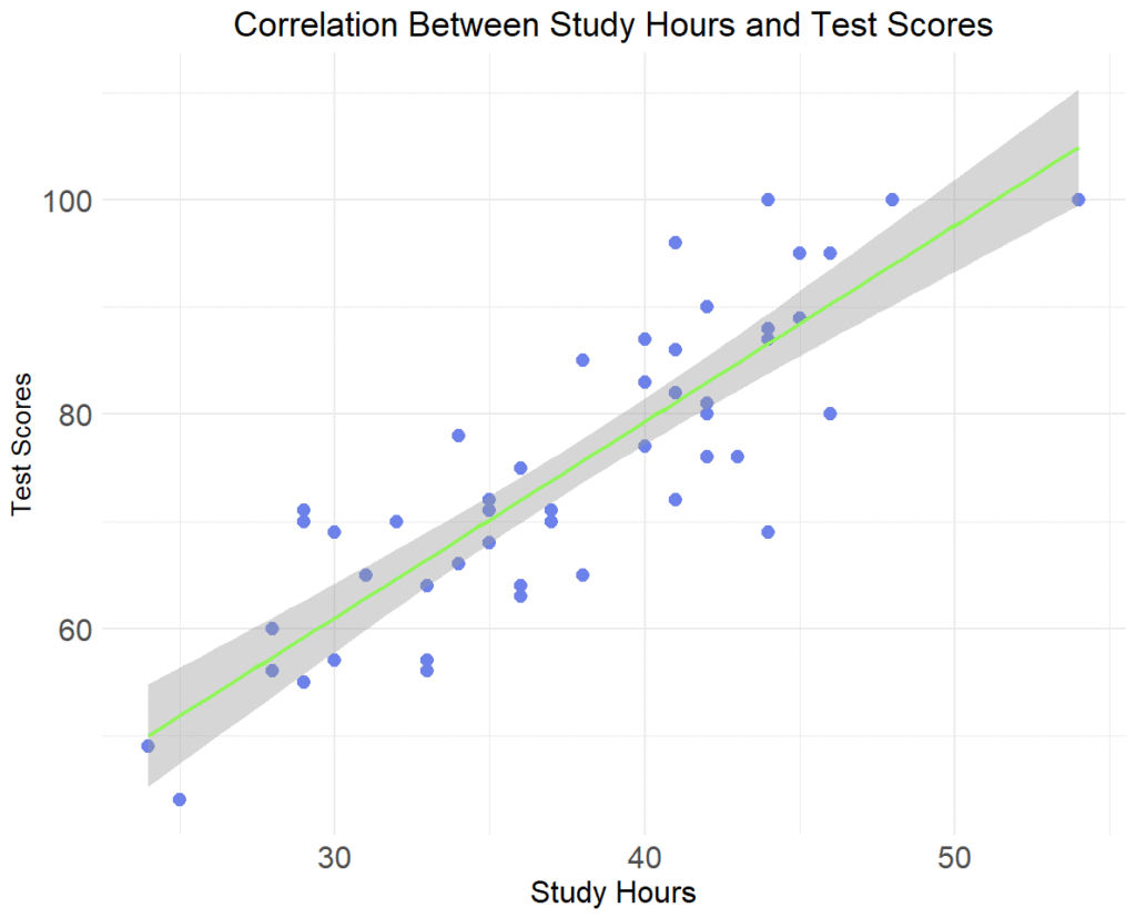
Figure 1 shows a scatter plot of the relationship between Study hours and Test scores. As we can see, as the number of study hours increases, the test scores also increase. The trend line shows a smoothed relationship line showing the average relationship between Study hours and Test scores. The next step is to perform a Pearson correlation to determine if the relationship between Study hours and Test scores is statistically significant.
To calculate a Pearson correlation between the study hours and test score, we use the cor.test() function in R. The cor.test() is a built-in R function, and therefore, we do not need to install and call a package to use this function. The following code in Listing 1 shows how to perform a Pearson correlation between two continuous random variables (study hours and test scores, in our example).
> dfScores <- read.csv("dsStudyHoursScores.csv")
> studyHours <- dfScores$Study_hours
> testScores <- dfScores$Score

> corrHoursScores <- cor.test(studyHours, testScores,
                            method = "pearson",
                            alternative = "two.sided")

> print(corrHoursScores)

	Pearson's product-moment correlation

data:  studyHours and testScores
t = 11.797, df = 48, p-value = 8.648e-16
alternative hypothesis: true correlation is not equal to 0
95 percent confidence interval:
 0.7683581 0.9198556
sample estimates:
      cor
0.8622877 In this code, the parameters of the cor.test() function include the names of the two variables (study hours and test scores), the statistical method (we asked for Pearson correlation), and the null hypothesis (two-sided, which means the null hypothesis, i.e., no relationship, while alternative hypothesis assumes there is correlation on either side, positive or negative).
The results of the Pearson correlation include the t value (because the Pearson correlation coefficient is distributed as a T distribution), the degree of freedom, the p-value, the 95% confidence interval of the correlation coefficient, and the correlation coefficient itself (shown as sample estimates: cor). In this example, the Pearson correlation is 0.86, it is positive, and statistically significant. This implies that there is a very strong relationship between the number of hours dedicated to studying and the test scores students achieve on the test. In other words, the more time dedicated to study, the higher the test score will be. The 95% confidence interval implies that for 95% of the times, the population correlation between the number of hours dedicated to studying and the test scores students achieve on the test falls between 0.77 and 0.92.