STATISTICS with R
A comprehensive guide to statistical analysis in R
Multiple Regression in R
Multiple regression is a statistical method that measures and models the relationship between two or more independent variables and one continuous dependent variable. The independent variables can be continuous, binary, or categorical. Modeling in multiple regression involves obtaining an equation from data that incorporates multiple predictors to better explain or predict a future outcome. Multiple regression is a fundamental method in predictive modeling, often used when the dependent variable is influenced by multiple factors simultaneously.
Introduction to Multiple Regression
We learned about regression in the simple linear regression module. A simple linear regression is used to model the relationship between one independent variable and the dependent variable. Such a simple linear regression could provide an acceptable fitted model to explain the relationship between the independent variable and the dependent variable (for example, by looking at the value of the R²). However, a single independent variable may not provide enough information to predict the dependent variable and may leave some unexplained variance in the dependent variable.
One way to add more information and reduce the unexplained variance in the dependent variable is to add more relevant independent variables based on theory, prior research, or expert opinion. For example, exercise may be a good predictor of weight loss, but including diet can also contribute to predicting weight loss. In other words, instead of a simple linear regression, we can use multiple linear regression to evaluate independent variables that predict weight loss.
Like a simple linear regression, the dependent variable in a multiple linear regression is continuous (measured on an interval or a ratio scale of measurement). However, the independent variables can be continuous, binary (two levels, like sex: male and female), or categorical (more than two levels, such as income: low income, middle income, and high income).
In multiple linear regression, one assumption is that the independent variables (predictors) are not highly correlated with each other. If the independent variables are highly correlated, the estimated regression coefficients will be unstable due to inflated variance. In addition, because of the high correlation of the independent variables, we cannot exactly infer the effect of the individual independent variables. The problem of highly correlated independent variables in multiple regression is called multicollinearity or collinearity problem. Therefore, we must make sure our independent variables are not highly correlated with each other. We can test for the existence of multicollinearity using correlation tests among independent variables, or use an index called variance inflation factor (VIF).
In the following sections, we introduce an example data set and demonstrate how to model the relationship between the independent and the dependent variable through a multiple regression in R.
Multiple Regression Example
What is the relationship between the number of hours students study, students academic motivation and their test scores? Can the number of studying hours and academic motivation predict test scores?

A high school teacher is interested in modeling the relationship between the number of hours students study and their academic motivation and the scores the students achieve on a test. The teacher randomly selects 65 students from the school district and asks the students how much time they dedicated to preparing for the test. In addition, the teacher administers a questionnaire on academic motivation to understand how motivated the students are. The teacher is not only interested in understanding the relationship between study hours and academic motivation and test scores, but also if the number of studies the and the motivation of students can be used to predict a student’s test score. Table 1 includes the scores of five students on the test along with the number of hours they studied and their motivation score on 0-100 scale.
| Student | Study Hours | Motivation Score | Test Score |
|---|---|---|---|
| Student 1 | 35 | 74 | 84 |
| Student 2 | 37 | 69 | 81 |
| Student 3 | 32 | 47 | 58 |
| Student 4 | 39 | 63 | 80 |
| Student 5 | 46 | 56 | 85 |
| … | … | … | … |
The teacher enters the data in a spreadsheet program in the school computer lab and saves the data in the CSV format. The complete data set for this example can be downloaded from here.
Analysis: Multiple Regression in R
In the first step, data are read into the RStudio program using the read.csv() function. In this example, the dependent variable is the students test scores, and the independent (predictor) variables are the number of study hours and the motivation scores of students. Mathematically, we read such relationship as “test score is a function of study hours and motivation”, or “test score depends on study hours and motivation”. In mathematical notation, we write it as: test score ~ study hours + motivation. Similar mathematical formulation is used in R language to show the relationship between a dependent variable and the independent variables. The dependent variable is written on the left-hand side of the equation, and the independent variables are written on the right-hand side of the equation.
To conduct a multiple linear regression between the test scores and study hours and motivation, we use the lm() function in R, which stands for linear modeling. The lm() function is a built-in function in base R (stats), and therefore, we do not need to install and call a package to use this function. We use the function notation (~) to show the relationship between the dependent variable (on the left-hand side) and the independent variables (on the right-hand side). The R code in Listing 1 shows how to perform a multiple linear regression to model the relationship between one dependent continuous random variable (test scores) and two independent continuous random variables (Study hours and Motivation).
To perform a simple linear regression between the test scores and study hours, we use the lm() function in R. The lm() function is a built-in R function, and therefore, we do not need to install and call a package to use this function. We use the function notation (~) to show the relationship between the dependent variable (on the left-hand side) and the independent variable (on the right-hand side). The following R code in Listing 2 shows how to perform a simple linear regression between to model the relationship between two continuous random variables (study hours and test scores, in our example).
> dfScores <- read.csv("dsMotivation.csv")

> mregStudyScores <- lm(testScore ~ studyHours + motivation, data = dfScores)
> summary(mregStudyScores)


Call:
lm(formula = testScore ~ studyHours + motivation, data = dfScores)

Residuals:
    Min      1Q  Median      3Q     Max
-8.3629 -2.5036 -0.3413  2.5644 10.5882

Coefficients:
            Estimate Std. Error t value Pr(>|t|)
(Intercept) -17.4900     4.2390  -4.126 0.000112 ***
studyHours    1.7786     0.1061  16.764  < 2e-16 ***
motivation    0.4365     0.0342  12.761  < 2e-16 ***
---
Signif. codes:  0 ‘***’ 0.001 ‘**’ 0.01 ‘*’ 0.05 ‘.’ 0.1 ‘ ’ 1

Residual standard error: 3.778 on 62 degrees of freedom
Multiple R-squared:  0.8866,	Adjusted R-squared:  0.883
F-statistic: 242.5 on 2 and 62 DF,  p-value: < 2.2e-16
In this code, the parameters of the lm() function include the name of the dependent variable (test score), the name of the independent variables (study hours and motivation), and the name of the data set the two variables are in. The model and its parameters are given a name, mregStudyScores (any arbitrary name). In this way, we create an object called mregStudyScores in the RStudio environment which carries several data and information bits, such as model formula and the results of the analysis. Therefore, we need another function to extract the desired information from the model object, such as summary(). This is the preferred way of building the model because later we may need to build another model and then compare the two models (for example, compare this current multiple regression model with two independent variables with a simple linear regression that includes only one of the independent variables).
The multiple linear regression results from the lm() function modeling the relationship between test scores and study hours and motivation are included in Listing 1. In the analysis output, the Call line shows our model. Residuals show the difference between what our model predicts against the truth (i.e., actual data). The coefficients are the most important information we are interested in. The intercept is the point on the z-axis (dependent variable) where the plain of best fits crosses (and where the x values, or the independent variable values are zero). In our example, the intercept is -17.490, meaning that when study hours is zero and motivation is none, we theoretically expect the test score to be -17.490. The next line in the Coefficients shows the coefficients for (effects of) the two independent variables “study hours” and “motivation”, which are 1.778 and 0.436, respectively, and which are both positive, and which are both statistically significant.
In a multiple linear regression, individual coefficients for an independent variable are interpreted with regard to the other independent variable. For example, the coefficient for the “study hours” is interpreted as follows: for each additional hour of study, the test score increases on average 1.778 scores controlling for the Motivation variable. By controlling for Motivation we mean keeping the Motivation variable at a fixed value and changing the study hours value freely. We demonstrate this concept in the following equation.
According to the results from the multiple linear regression example,
Expected test score = -17.490 + 1.778 *(study hours) + 0.436*(motivation).
The equation above is our model and we can use it to predict a test score if we have information about the number of study hours. For example, if an individual studies for 40 hours a week and whose motivation score is 86, we predict their test score to be:
Expected test score = -17.490 + 1.778 *(40) + 0.436*(86) = 91.126
Now let’s explore what we mean by “for each additional hour of study, the test score increases on average 1.778 scores controlling for the Motivation variable.” In the example above, hours of study value was set to 40. Now, for each additional hour of study, such as one hour, the test score increases on average 1.778 scores controlling for motivation. And we said “controlling for” means fixing the other variable at a constant value, such as 86 in example above. Let’s calculate the new score for one additional hour of study (41) but the same motivation value (86, controlled for):
Expected test score = -17.490 + 1.778 *(41) + 0.436*(86) = 92.904
We can see that the test score increased to 92.904 for one additional hour of study and keeping the motivation unchanged (controlled for). The increase in score is: 92.904 – 91.126 = 1.778, which is the coefficient of the Study hours variable in the R results. We can argue the same for one unit change in Motivation, controlling for Study hours, which increases the test score by 0.436.
In the remainder of the output, the Adjusted R-squared value of 0.883 in the last line of the results shows that the linear combination of Study hours and Motivation accounts for 88% of the variance in the dependent variable. In other words, Study hours and Motivation contribute 88% of the information we need to predict the values in the test scores. Adjusted R-squared can be used as a measure of model adequacy (not model fit). It shows whether we have enough information in our independent variables, or we whether need to replace or supplement them with other independent variables. R-squared is adjusted (penalized) because as we add more independent variables and the sample size increases, the R-squared value artificially inflates.
As stated in the introductory section of this chapter, the independent variables in our regression model could be highly correlated and cause multicollinearity problem. We can check for the existence of the multicollinearity problem by conducting the variance inflation factor (VIF), which measures how much the variance in the regression coefficients is inflated because of the high correlation in the independent variables. Ideally, we want our VIF value to be 1 (i.e., zero correlation between the independent variables). VIF values less then 5 are acceptable and show that the independent variables are weakly correlated. After running a regression model, we can conduct a VIF procedure. In R, we can use the package car and the function vif() to calculate the VIF values (you may need to install the package if it is not installed on your computer). The input to the vif() function is the name of the multiple regression model we conducted above (“mregStudyScores”). Listing 2 includes the R code to calculate VIF for our model above.
> dfScores <- read.csv("dsMotivation.csv")

> mregStudyScores <- lm(testScore ~ studyHours + motivation, data = dfScores)

# Calculate Variance Inflation Factor (VIF)
> library(car)
> vif(mregStudyScores)

studyHours motivation
   1.00768    1.00768
In Listing 2, the VIF value for the collinearity between Study hours and Motivation is 1.007, which is very close to 1. We can conclude that our model does not have multicollinearity problem.
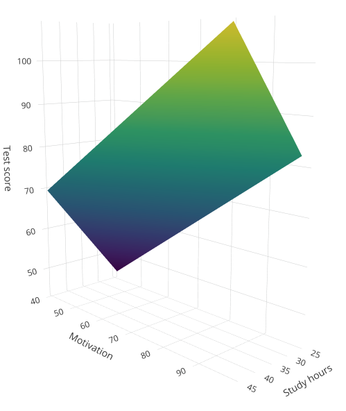
Figure 1 below shows the relationship between Study hours and Motivation with Test scores modelled through multiple regression.