STATISTICS with R
A comprehensive guide to statistical analysis in R
Measures of Dispersion in R
Measures of dispersion are values that indicate how spread out or concentrated data points are, summarizing the variation within a dataset. They help determine whether the data distribution deviates from an expected shape, contains anomalies, or includes all possible cases. These measures are also frequently applied in other statistical methods for normalizing data and calculating additional statistics. Common measures of dispersion in descriptive statistics include range, interquartile range, variance, and standard deviation. In research reports, measures of dispersion are typically presented alongside measures of central tendency as part of descriptive statistics.
Range
The range of a data set is the difference between its highest (maximum) and lowest (minimum) values. Since it spans the entire set, it’s a measure of how spread out the data is. For example, if the range of blood pressure in female patients is 20 and in male patients is 15, it shows there’s less variation in the male data. A large range might suggest extreme values or possible data entry mistakes. The range is calculated as:
One application of range is data normalization, also known as scaling, where the scale of the data changes through transformation, particularly in machine learning. When data has a large spread, adjusting it by its range, defined by the difference between the maximum and minimum values, enhances the robustness of analysis results. Min-max normalization or scaling incorporates the range in the denominator using the following formula:
Interquartile Range
While the range is a single value representing the span of the entire data distribution, the interquartile range (IQR) measures dispersion within the middle portion of the data, specifically the middle 50% when sorted. The IQR is calculated as the difference between the third and first quartiles, indicating the spread of the central half of the dataset. Because there are different methods to calculate the quartiles, different methods and software may produce slightly different values for interquartile range. Interquartile range is useful for detecting outliers, describing skewed distributions, and summarizing ordinal variables. One application, known as the Tukey Outlier Rule, uses the IQR in a formula to identify outliers in a distribution.
Interquartile range is useful for detecting outliers, describing skewed distributions, and summarizing ordinal variables. One application, known as the Tukey Outlier Rule, uses the IQR in a formula to identify outliers in a distribution.
Values outside this range are treated as outliers.
Note: Different software (e.g., SPSS, Minitab, SAS, R) may use different methods to compute interquartile range and their values may differ slightly.
Variance
Variance is an important measure of dispersion in a distribution, indicating how far values deviate from the mean by averaging the squared deviations. A small variance suggests that data points are close to the mean, while a large variance indicates they are more spread out. Variance serves as a foundational concept for many statistical measures, including standard deviation, and methods such as analysis of variance (ANOVA). In a sample data set, variance is calculated as follows:
Because the distance between each data point and the mean is squared in the process of calculating the variance, the value of variance is not on the same scale as the original data distribution.
Standard Deviation
The most common measure of dispersion for data that is approximately normally distributed is the standard deviation. It represents the average deviation of data points from the mean and is expressed on the same scale as the original data, unlike variance. A small standard deviation indicates that data points are closely clustered around the mean, while a large one reflects greater spread. The sample standard deviation is calculated by taking the square root of the sample variance:
Standard deviation is a key measure in statistical analysis, used for describing distributions, assessing model assumptions, detecting outliers, and comparing variability between groups. Outliers can be identified by observations that fall several standard deviations from the mean, often beyond ±3 SD, where such values are statistically improbable in an approximately normal distribution.
Calculating Range, Interquartile Range, Variance, and Standard Deviation in R
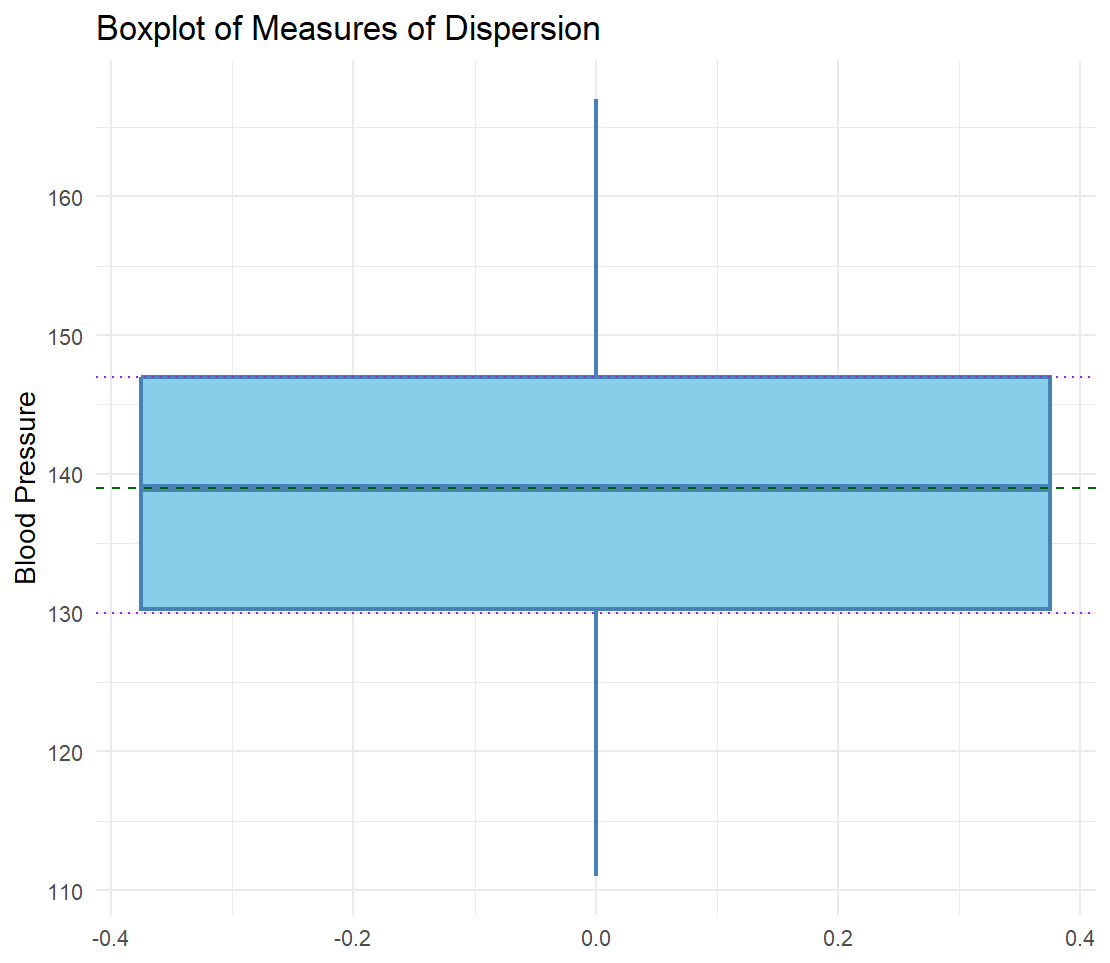
We demonstrate how the range, interquartile range, variance, and standard deviation of a variable (measures of dispersion) are calculated in R using a blood pressure measurement dataset. The dataset can be download as CSV format. The data includes blood pressure measurements of 30 patients at two time points (BP01 and BP02). We are interested in knowing the range, interquartile range, the variance, and the standard deviation of blood pressure measurements at Time 1 (BP01). Listing 1 provides the R code to compute the measures of dispersion. Note: The built-in R function range() outputs the the maximum and minimum values, not their difference; we write a custom function to compute the range.
# Blood pressure data
dfBloodPressure <- read.csv("dsCardamom.csv")

# Blood pressure at time 1
BPTime01 <- dfBloodPressure$Before

# Custom function to compute range
getRange <- function(v, na.rm = TRUE) {
     if (na.rm) v <- v[!is.na(v)]
     maxV <- max(v)
     minV <- min(v)
     rangeV <- maxV-minV
     return(rangeV)
}

# Range, IQR, variance, SD
getRange(BPTime01)
IQR(BPTime01, type = 7) # Used by R
IQR(BPTime01, type = 6) # Used by SPSS
var(BPTime01)
sd(BPTime01)

getRange(BPTime01)
56
IQR(BPTime01, type = 7) # Used by R
16.75
IQR(BPTime01, type = 6) # Used by Minitab and by SPSS
18.25
var(BPTime01)
214.2483
sd(BPTime01)
14.63722
The results in Listing 1 show that the range of blood pressure is 56, the IQR is 16.75, and the variance is 214.25, and the standard deviation is 14.64.