STATISTICS with R

Measures of central tendency are statistical values that represent the typical or most frequent point in a distribution, indicating where other data points tend to cluster. They offer a concise summary of the overall distribution. The most common measures of central tendency are the mean, median, and mode. In research papers, these values are typically presented in the descriptive or exploratory statistics section, often in a table referred to as the Table 1 and are usually reported alongside measures of dispersion.

When data is measured on a ratio or interval (continuous) scale, the mean is one of the most useful pieces of summary information about its distribution. It is directly applied in certain statistical methods, such as t-tests for comparing means between two groups of participants. Also referred to as the average, arithmetic mean, or expected value, the mean is calculated by summing the values of a variable (distribution) and dividing the total by the number of values.

For example, a researcher has collected the following blood pressure measurements from five patients: [132, 137, 163, 141, 141]. The mean blood pressure is

The mean is a useful summary statistic when there aren’t any extreme values in the distribution, since outliers can skew it as a measure of central tendency. These extreme values pull the mean away from the center, especially in smaller samples. In such situations, it’s better to report the median.

Another measure of central tendency is the median, which represents the value in a data set that divides the ordered distribution into two equal halves. In other words, 50% of the values lie below the median and 50% lie above it. For this reason, the median is also called the 50th percentile ($P_{50}$). The median is a useful summary statistic when the distribution contains extreme values or is not symmetrical. For example, in reporting housing property values, the median is often used because some property values can be significantly higher than those of a typical home.

The median of a data distribution can be located by first sorting the data from smallest to the greatest, and then finding the middle value (for odd number of data points). If there are an even number of data points (e.g., 10 blood pressures measurements), the median is defined to be the average of the two middle values (i.e., the average of the fifth and the sixth ordered values). For example, for the following 11 blood pressure measurements [132, 137, 163, 141, 141, 142, 166, 147, 121, 130, 133], first we sort them: [121, 130, 132, 133, 137, 141, 141, 142, 147, 163, 166], and find the middle value as the median, which is 141.

For the following sorted 10 blood pressure measurements, [121, 130, 132, 133, 137, 141, 141, 142, 147, 163], since there are even (10) numbers, the median is the average of the 5th and 6th values: (137 + 141) / 2 = 139.

In a data distribution, certain values may occur multiple times. The value with the highest frequency of occurrence is called the mode of the distribution. For instance, in a set of blood pressure measurements, the value 142 might appear most often. In a survey, one option may be selected more frequently than others, indicating the mode. If two values occur with the same highest frequency, the distribution is considered bimodal. For example, if blood pressure readings of 142 and 130 each appear seven times, the distribution has two modes and is classified as bimodal.

The mean and the median of a distribution can be calculated with R base functions mean() and median(). In addition, some packages provide summary functions that provide additional descriptive statistics. However, currently R does not provide a built-in function to find the modes of a distribution. So, we need to write our own custom function to find the mode(s) of a distribution.

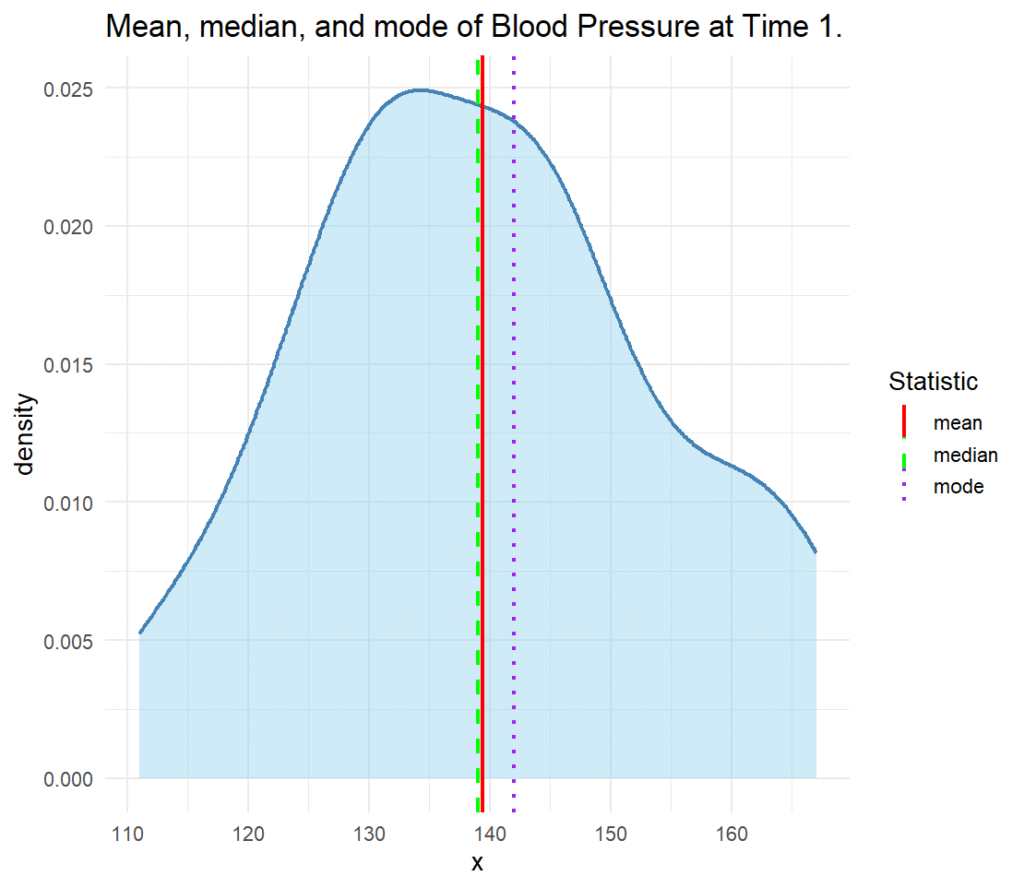
We demonstrate how the mean, the median, and the mode of a variable (measures of central tendency) are calculated using the blood pressure measurement dataset. The dataset can be download from this link in CSV format. The data includes blood pressure measurements of 30 patients at two time points (BP01 and BP02). We are interested in knowing the mean, the median, and the mode of blood pressure measurements at time 1 (BP01). Listing 1 shows the R code for calculating the mean, the median, and the mode of blood pressure measurements.

# Blood pressure data 
dfBloodPressure <- read.csv("dsCardamom.csv")

# Blood pressure at time 1
BPTime01 <- dfBloodPressure$Before 

# Custom function to get mode(s)
getModes <- function(v, na.rm = TRUE) {
     if (na.rm) v <- v[!is.na(v)] # remove NA if TRUE
     tab <- table(v)
     maxFreq <- max(tab)
     modes <- names(tab)[tab == maxFreq]
     return(modes)
}

# Mean, median, mode
mean(BPTime01)
[1] 139.4
median((BPTime01))
[1] 139
getModes(BPTime01)
[1] "142"

# Blood pressure data 
dfBloodPressure <- read.csv("dsCardamom.csv")

# Blood pressure at time 1
BPTime01 <- dfBloodPressure$Before 

# Custom function to get mode(s)
getModes <- function(v, na.rm = TRUE) {
     if (na.rm) v <- v[!is.na(v)] # remove NA if TRUE
     tab <- table(v)
     maxFreq <- max(tab)
     modes <- names(tab)[tab == maxFreq]
     return(modes)
}

# Mean, median, mode
mean(BPTime01)
[1] 139.4
median((BPTime01))
[1] 139
getModes(BPTime01)
[1] "142"

The results in Listing 1 show that the mean blood pressure is 139.4, the median is 139, and the mode is 142.