STATISTICS with R

The Kaplan–Meier curve is a fundamental method in survival analysis, used to estimate the probability of surviving beyond a given time while accounting for censored observations. As part of survival analysis—a branch of statistics focused on modeling time-to-event data—the Kaplan–Meier approach allows us to visualize how survival probabilities change over time and to compare these probabilities across different groups. Survival analysis also investigates which variables or characteristics influence the occurrence of events, often extending to methods such as Cox regression for assessing risk factors. Typical time-to-event outcomes include death, mechanical or electrical failure, seed germination, property sales, or the time until a drug becomes effective.

In some studies, we are interested in modeling the time it takes for the occurrence of an event. The outcome in these data is the status of an event, such as death from cancer, failure of a mechanical heart valve, wear of vehicle tires, and relapse to smoking. Such data are generally named time-to-event data and the statistical methods used to model these data are commonly called survival analysis. Survival analysis models describe the lifetime of individuals (e.g., cancer patients) or duration of events (e.g., time to failure of a mechanical heart or hip replacement or dental implants). In addition, survival models help us understand if the distribution of survival times is identical across groups, such as between female and male patients, treatment methods, or device materials.

The data in a survival analysis has two outcomes: event (cases that experienced the event) and censored (cases that did not experience the event). What makes the survival data different from a binary outcome distribution is the presence of cases which have not experienced the event of interest (e.g., death, failure, relapse) during or after the time frame in which data is collected. For example, in a study on a new drug, the effectiveness of drug is followed up for 12 months. Some patients may drop out and some patients may not show any improvement during the 12-month period. However, we are not sure what happens to those patients who drop out or cannot be followed up after 12 months. As another example, in a study on time-to-germination of seeds, some seeds may be eaten by birds and therefore we do not know their time to germination. Or a property owner may remove their listing from the market, and we do not know how long it would have taken to sell. Such cases are called censored observations and must be included in the analysis.

Survival analysis methods, such as Kaplan-Meier, address this incompleteness (censored observations) in data. Censored observations also include those cases that we know did not experience the event (e.g., did not die, did not break, etc.). The Kaplan-Meier curve is a step function that displays the probability of survival over time, taking into account censored data (e.g., patients who leave the study or are lost to follow-up).

In the following sections, we present an example research scenario where a survival analysis using Kaplan-Meier method will be used to analyze the data. We will demonstrate how to perform survival analysis using Kaplan-Meier method in SPSS step-by-step. In a separate module, we present Cox (proportional hazard) regression to investigate what factors influence survival probability.

What is the survival probability of a patient with primary brain tumor after 24 months of receiving therapy? Is the survival probability equal across male and female patients? Is the survival probability equal across different treatment methods?

A team of doctors and health researchers are interested in understanding the survival probability of primary brain tumor patients receiving treatment with different stereotactic radiation methods at a cancer institute (Masaryk Memorial Cancer Institute Brno). In addition, the researchers are interested in any difference in the effectiveness of the treatment between female and male patients and treatment methods.

For this purpose, the researchers collected data from 88 primary brain tumor patients on their sex (male, female), gross tumor volume (GTV), tumor diagnosis (meningioma, LG glioma, HG glioma, others), the location of the tumor in the brain (infratentorial or supratentorial), Karnofsky index (an index showing health, ranging from excellent health 100% to very poor health 0%), and treatment methods (SRS or SRT). The two treatment methods include SRS (stereotactic radiosurgery) or SRT (stereotactic radiotherapy). The event of interest in this survival analysis was the death of the patients, shown in the status variable (1 = dead, 0 = censored). Time to the event is shown in the time variable (months). Table 1 shows data for five patients in this study.

The data for this example can be downloaded in the CSV format. The data is also available in the supplemental file of the published paper.

In a survival analysis, we try to find the probability of survival for a patient after a certain amount of time in a follow-up. In addition, if there is a grouping variable in the data, such as sex, treatment method, or dosage, survival analysis can also address the question if such a survival probability is different across the groups or a continuous covariate, such as dosage. These questions can be addressed using the Kaplan-Meier method (for producing the survival probability curve over time period) and the log-rank test (for testing group difference). If we are also interested in knowing the effect of an independent variable (risk factor) on the survival probability, we can use a regression method called Cox proportional hazard regression.

In our example data, we are interested in obtaining survival probability curve estimate (also known as Kaplan-Meier curve) and investigating if the survival probability is different across sex (using log-rank test).

First we install and load the required R packages for survival analysis. The packages needed to perform Kaplan-Meier curve estimation in R are survival and survminer (for plotting) packages. Installation of a package in RStudio is explained in chapter First Time Installation of R and RStudio. Listing 1 shows the R code to run Kaplan-Meier curve estimation.

library(survival)
library(survminer)

# Data: Brain cancer patients survival times
dfBrainCancer <- read.csv("dfBrainCancer.csv")


# All patients together
mdAllSurvCancer <- survfit(Surv(time, status) ~  1, data = dfBrainCancer)
print(mdAllSurvCancer)
Call: survfit(formula = Surv(time, status) ~ 1, data = dfBrainCancer)

      n events median 0.95LCL 0.95UCL
[1,] 88     35   47.8    33.4      NA


summary(mdAllSurvCancer)
Call: survfit(formula = Surv(time, status) ~ 1, data = dfBrainCancer)

  time n.risk n.event survival std.err lower 95% CI upper 95% CI
  0.07     88       1    0.989  0.0113        0.967        1.000
  1.41     86       1    0.977  0.0160        0.946        1.000
  3.38     83       1    0.965  0.0197        0.928        1.000
  4.16     82       1    0.954  0.0227        0.910        0.999
  4.56     81       1    0.942  0.0253        0.894        0.993
  

library(survival)
library(survminer)

# Data: Brain cancer patients survival times
dfBrainCancer <- read.csv("dfBrainCancer.csv")


# All patients together
mdAllSurvCancer <- survfit(Surv(time, status) ~  1, data = dfBrainCancer)
print(mdAllSurvCancer)
Call: survfit(formula = Surv(time, status) ~ 1, data = dfBrainCancer)

      n events median 0.95LCL 0.95UCL
[1,] 88     35   47.8    33.4      NA


summary(mdAllSurvCancer)
Call: survfit(formula = Surv(time, status) ~ 1, data = dfBrainCancer)

  time n.risk n.event survival std.err lower 95% CI upper 95% CI
  0.07     88       1    0.989  0.0113        0.967        1.000
  1.41     86       1    0.977  0.0160        0.946        1.000
  3.38     83       1    0.965  0.0197        0.928        1.000
  4.16     82       1    0.954  0.0227        0.910        0.999
  4.56     81       1    0.942  0.0253        0.894        0.993
  

The function Surv requires the time and survival status arguments. Survival status is a variable that shows if the patient died (event= 1) or survived / censored (event = 0). The time variable shows how long after follow-up the patient died. In the formula notation Surve(time, status) ~ 1, we indicate that we are interested in estimating the Kaplan-Meier curve for all patients regardless of their sex, treatment, age, and any other grouping variable. If we are interested in comparing the Kaplan-Meier curve across groups, like sex, we replace 1 with the name of the grouping variable (e.g., sex).

The median survival time for all patients combined is 47.8 months, as shown in Listing 1. In survival analysis, the median survival time is generally reported because of the skewed nature of the data distribution. Calculation of median survival in Kaplan-Meier estimation is different from arithmetic calculation of median. Therefore, in reporting the median survival time, we must always report the median survival time calculated from the fitted survival model. In addition, we can see the total number of patients is 88 and the total number of events (deaths) is 35.

In Listing 1 code, we can also see the summary of the survival function fitted by calling the summary function. In the output, we can see the time, number at risk at the time, number of events (death), the survival probability at the time, the standard error, and the lower and upper confidence interval of the survival probability. For example, at time 0.07 (month), 88 patients were at risk, out which 1 patient died. So, the survival probability at this time is 0.989. At time 1.41, 86 patients remained (number at risk), and at this time 1 more patient died (two patients overall dies at this time, hence the number at risk decreased from 88 to 86). At this time, the survival probability is 0.977.

We can plot the survival probability over time from the table using the base plot function or the ggsurvplot function from the survminer package. Listing 2 shows the R code for plotting the survival probability for the brain cancer patients in this study.

library(survival)
library(survminer)

# Data: Brain cancer patients survival times
dfBrainCancer <- read.csv("dfBrainCancer.csv")

# All patients together
mdAllSurvCancer <- survfit(Surv(time, status) ~  1, data = dfBrainCancer)

# Plot Kaplan-Meier Curve
ggsurvplot(mdAllSurvCancer, data = dfBrainCancer,
           title = "Survival Probability of Brain Cancer Patients",
           conf.int = FALSE,
           risk.table = TRUE,
           break.time.by = 5,
           ggtheme = theme_light())

library(survival)
library(survminer)

# Data: Brain cancer patients survival times
dfBrainCancer <- read.csv("dfBrainCancer.csv")

# All patients together
mdAllSurvCancer <- survfit(Surv(time, status) ~  1, data = dfBrainCancer)

# Plot Kaplan-Meier Curve
ggsurvplot(mdAllSurvCancer, data = dfBrainCancer,
           title = "Survival Probability of Brain Cancer Patients",
           conf.int = FALSE,
           risk.table = TRUE,
           break.time.by = 5,
           ggtheme = theme_light())

We can adjust several parameters in the ggsurvplot function, such as time axis units and adding confidence intervals. The plot in Figure 1 shows the Kaplan-Meier curve estimates of survival probability and the number of patients at risk (remaining patients) at different time points. If we know how long a patient has been in the treatment plan, we can estimate their survival probability. For example, for a patient in the treatment plan for 40 months, their survival probability is about 0.55 (which can also be read from the Survival Table). The plus signs on the curve indicate censored cases.

In survival analysis, we may also be interested in understanding if the survival probability is different between groups, such as sex or treatment groups. Listing 3 shows the R code to run Kaplan-Meier curve estimation and plot for female and male patients.

library(survival)
library(survminer)

# Data: Brain cancer patients survival times
dfBrainCancer <- read.csv("dfBrainCancer.csv")

# Female and male patients
mdSexSurvCancer <- survfit(Surv(time, status) ~  sex, data = dfBrainCancer)
print(mdSexSurvCancer)
Call: survfit(formula = Surv(time, status) ~ sex, data = dfBrainCancer)

            n events median 0.95LCL 0.95UCL
sex=Female 45     15   51.0    46.2      NA
sex=Male   43     20   31.2    20.7      NA

summary(mdSexSurvCancer)

# Plot Kaplan-Meier Curve
ggsurvplot(mdSexSurvCancer , data = dfBrainCancer,
           title = "Survival Probability of Brain Cancer Patients by Sex",
           conf.int = FALSE,
           risk.table = TRUE,
           break.time.by = 5,
           ggtheme = theme_light())

library(survival)
library(survminer)

# Data: Brain cancer patients survival times
dfBrainCancer <- read.csv("dfBrainCancer.csv")

# Female and male patients
mdSexSurvCancer <- survfit(Surv(time, status) ~  sex, data = dfBrainCancer)
print(mdSexSurvCancer)
Call: survfit(formula = Surv(time, status) ~ sex, data = dfBrainCancer)

            n events median 0.95LCL 0.95UCL
sex=Female 45     15   51.0    46.2      NA
sex=Male   43     20   31.2    20.7      NA

summary(mdSexSurvCancer)

# Plot Kaplan-Meier Curve
ggsurvplot(mdSexSurvCancer , data = dfBrainCancer,
           title = "Survival Probability of Brain Cancer Patients by Sex",
           conf.int = FALSE,
           risk.table = TRUE,
           break.time.by = 5,
           ggtheme = theme_light())

According to the results in Listing 3, the median survival time for female patients is 51.0 months while that of male patients is 31.2 months (male patients were more likely to die at a given time). Figure 2 shows the separate Kaplan-Meier curves for female and male patients.

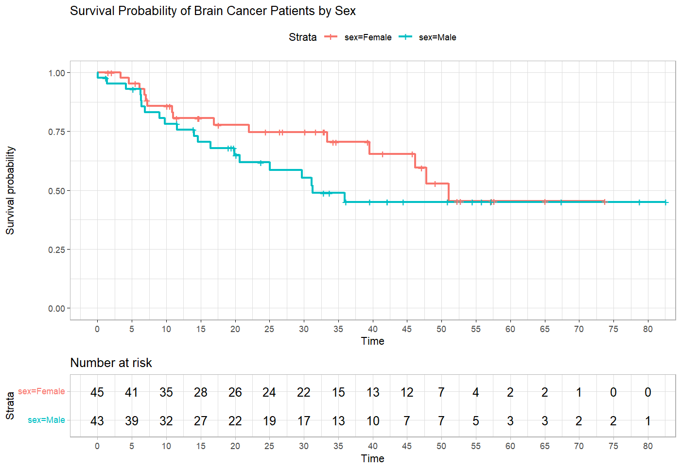
According to Figure 2, we can see that at most time points, male patients have lower survival probability than female patients. However, the difference becomes negligible after about 50 months. The risk table also shows that after time 50 (months), the number of patients at risk remains similar in both female and male patients. We test for the statistical significance of the difference in survival probability between female and male patients using log-rank test.

The log-rank test is based on the chi-square statistic and distribution. The log-rank test in survival analysis can be used to test the statistical significance of difference between survival probabilities of different groups. In this example, we use the log-rank test to see if the survival probability is different between female and male patients. Listing 4 includes the R code to run the log-rank test using the survdiff function.

library(survival)
library(survminer)

# Data: Brain cancer patients survival times
dfBrainCancer <- read.csv("dfBrainCancer.csv")

# Log-rank test for sex difference
lrTest <- survdiff(Surv(time, status) ~ sex, data = dfBrainCancer)
print(lrTest)

Call:
survdiff(formula = Surv(time, status) ~ sex, data = dfBrainCancer)

            N Observed Expected (O-E)^2/E (O-E)^2/V
sex=Female 45       15     18.5     0.676      1.44
sex=Male   43       20     16.5     0.761      1.44

 Chisq= 1.4  on 1 degrees of freedom, p= 0.2 

library(survival)
library(survminer)

# Data: Brain cancer patients survival times
dfBrainCancer <- read.csv("dfBrainCancer.csv")

# Log-rank test for sex difference
lrTest <- survdiff(Surv(time, status) ~ sex, data = dfBrainCancer)
print(lrTest)

Call:
survdiff(formula = Surv(time, status) ~ sex, data = dfBrainCancer)

            N Observed Expected (O-E)^2/E (O-E)^2/V
sex=Female 45       15     18.5     0.676      1.44
sex=Male   43       20     16.5     0.761      1.44

 Chisq= 1.4  on 1 degrees of freedom, p= 0.2 

According to the log-rank test results, there is not a statistically significant difference between female and male patients in terms of survival probability (chi-square = 1.4, df = 1, p = 0.2).