STATISTICS with R
A comprehensive guide to statistical analysis in R
Cox Regression in R
Cox regression is a widely used technique in survival analysis that models how the occurrence of an event relates to a set of explanatory variables. Unlike the Kaplan–Meier estimator or the log-rank test, which compare survival probabilities across groups, Cox regression allows for a multivariable perspective—examining how several predictors simultaneously influence the likelihood of the event. Because of its flexibility and interpretability, it has become one of the most common approaches in medical and health research for analyzing time-to-event data.

Introduction to Cox Regression
In survival analysis, the central goal is to model the time until a particular event occurs, such as death, recovery, or relapse. The Kaplan–Meier estimator provides a way to visualize survival probabilities over time, while the log-rank test is used to compare survival curves between groups. Cox regression extends these approaches by examining how multiple predictors—such as age, sex, or treatment type—affect the risk of the event. As one of the most widely applied methods in survival research, the Cox proportional hazards model offers valuable insight into how different factors shape patient outcomes.
Cox regression is considered a semi‑parametric approach because it does not require specifying a particular distribution for survival times. This flexibility makes it broadly useful across different types of data. The model produces hazard ratios (HRs) for each predictor, which represent the relative risk of the event occurring at any given time, conditional on that predictor. An HR greater than 1 suggests an elevated risk, while an HR below 1 indicates a reduced risk.
Key assumptions of Cox regression include the proportional hazards assumption, which states that the hazard ratios for the predictors are constant over time. This means that the effect of a predictor on the hazard is multiplicative and does not change as time progresses. It is important to check this assumption before interpreting the results of a Cox regression analysis. Cox regression can handle both continuous and categorical predictors, allowing for a comprehensive analysis of factors influencing survival. It can also accommodate censored data, which is common in survival analysis when the event of interest has not occurred for some subjects by the end of the study period.
In the following sections, we present an example research scenario where a Cox regression method will be used to analyze survival data. We will demonstrate how to perform and interpret Cox regression in R in a step-by-step way.
Cox Regression Example
What factors impact the survival probability of a patient with primary brain tumor? Do patients’ sex, tumor location, gross tumor volume, tumor type, patient healthiness index (Karnofsky index), and tumor treatment method have a significant relationship with survival probability?

To address this research question, a team of doctors and health researchers (Masaryk Memorial Cancer Institute Brno) collected data from 88 primary brain tumor patients on their sex (male, female), gross tumor volume (GTV), tumor diagnosis (meningioma, LG glioma, HG glioma, others), the location of the tumor in the brain (infratentorial or supratentorial), Karnofsky index (an index showing health, ranging from excellent health 100% to very poor health 0%), and treatment methods (SRS or SRT). The two treatment methods include SRS (stereotactic radiosurgery) or SRT (stereotactic radiotherapy). The event of interest in this survival analysis was the death of the patients, shown in the status variable (1 = dead, 0 = censored). Time to event is shown in the time variable (in months). Table 1 includes data for five patients in this study.
| Patient | Sex | Diagnosis | Location | Karnofsky Index | GTV | Treatment Method | Status | Time (m) |
|---|---|---|---|---|---|---|---|---|
| Patient 1 | Female | Meningioma | Infratentorial | 90 | 6.11 | SRS | 0 | 57.64 |
| Patient 2 | Male | HG glioma | Supratentorial | 90 | 19.35 | SRT | 1 | 8.98 |
| Patient 3 | Female | Meningioma | Infratentorial | 70 | 7.95 | SRS | 0 | 26.46 |
| Patient 4 | Female | LG glioma | Supratentorial | 80 | 7.61 | SRT | 1 | 47.8 |
| Patient 5 | Male | HG glioma | Supratentorial | 90 | 5.06 | SRS | 1 | 6.3 |
| … | … | … | … | … | … | … | … | … |
The complete data set for this example can be downloaded from here. The data is also available in the supplemental file of the published paper.
Analysis: Cox Regression in R
Cox regression can be performed in R using the coxph() function from the “survival” library installed be default in base R. Similar to the Kaplan-Meier curve estimate, first a survival object is created and then the Cox regression model is fit with the predictors of interest. In this study, we are interested in knowing the predictive effect of sex, diagnosis, cancer location, KI value, and treatment type on incidence of brain cancer. Because some of the variables are categorical, first we convert them to factor (another term for a categorical variable). In addition, we select a reference level (category) to compare all other categories within a variable against with. For example, for the variable sex, we choose Male as the reference level. Therefore, the results will show the coefficient for Female and we can compare it (in odd terms) against Male patients. Choosing a different reference level changes the sign (negative or positive) in a binary factor and may change both sign and values in a categorical variable, such as diagnosis. Listing 1 shows the R code to run Cox regression for survival of brain cancer patients to examine the conditional effect of each predictor.
library(survival)

## Data proeprocessing
dfBrainCancer <- read.csv("dfBrainCancer.csv", stringsAsFactors = FALSE)

# Variable Diagnosis has missing values enteres as -1; convert to NA
dfBrainCancer$diagnosis[dfBrainCancer$diagnosis == -1] <- NA

# Recast categorical variables to factors and set reference level for each factor
refLevel<- c(sex = "Male",
             diagnosis = "Other",
             location = "Supratentorial",
             treatment = "SRT")

for (col in names(refLevel)) {
  dfBrainCancer[[col]] <- relevel(factor(dfBrainCancer[[col]]),
  ref = refLevel[[col]])

## Cox regression
modCox <- coxph(Surv(time, status) ~ sex + diagnosis + location + KI + GTV + treatment,
                data = dfBrainCancer)
summary(modCox)
The results of the Cox regression analysis are shown in Listing 2 below.
Call:
coxph(formula = Surv(time, status) ~ sex + diagnosis + location +
    KI + GTV + treatment, data = dfBrainCancer)

  n= 87, number of events= 35
   (1 observation deleted due to missingness)

                           coef exp(coef) se(coef)      z Pr(>|z|)
sexFemale              -0.18375   0.83215  0.36036 -0.510  0.61012
diagnosisHG glioma      1.26887   3.55683  0.61767  2.054  0.03995 *
diagnosisLG glioma      0.02933   1.02976  0.80003  0.037  0.97076
diagnosisMeningioma    -0.88570   0.41243  0.65787 -1.346  0.17821
locationInfratentorial -0.44119   0.64327  0.70367 -0.627  0.53066
KI                     -0.05496   0.94653  0.01831 -3.001  0.00269 **
GTV                     0.03429   1.03489  0.02233  1.536  0.12466
treatmentSRS           -0.17778   0.83713  0.60158 -0.296  0.76760
---
Signif. codes:  0 ‘***’ 0.001 ‘**’ 0.01 ‘*’ 0.05 ‘.’ 0.1 ‘ ’ 1


                       exp(coef) exp(-coef) lower .95 upper .95
sexFemale                 0.8321     1.2017    0.4106    1.6863
diagnosisHG glioma        3.5568     0.2811    1.0600   11.9351
diagnosisLG glioma        1.0298     0.9711    0.2147    4.9399
diagnosisMeningioma       0.4124     2.4247    0.1136    1.4974
locationInfratentorial    0.6433     1.5546    0.1620    2.5548
KI                        0.9465     1.0565    0.9132    0.9811
GTV                       1.0349     0.9663    0.9906    1.0812
treatmentSRS              0.8371     1.1946    0.2575    2.7218

Concordance= 0.794  (se = 0.04 )
Likelihood ratio test= 41.37  on 8 df,   p=2e-06
Wald test            = 38.7  on 8 df,   p=6e-06
Score (logrank) test = 46.59 on 8 df, p=2e-07The output in Listing 2 contains the results of the Cox regression on brain cancer survival data. Similar to a logistic regression, we can see the coefficients on log-odds scale (in the “coef” column) and odds scale (in the “exp” columns). For example, the log-odds coefficient for Female patients (compared to reference level Male) is -0.184 on the log-odds scale and 0.83 on the odds scale (hazard ratio). We interpret this result as: compared to Male patients, the hazard ratio of Female patients is lower by about 17%. However, this difference is not statistically significant as shown by the p value (p = 0.61) and the confidence intervals [0.41, 1.69]. Also, as indicated by the p value and the confidence intervals, the hazard ratio of HG Glioma compared to the chosen reference category (Other diagnosis) is statistically significant. The effect of KI on survival is also statistically significant (for each unit increase in KI, hazard ratio decreases by about 5%.) Table 2 provides a summary of the Cox regression results.
| Predictor | Hazard Ratio (HR) | 95% CI | p-value | Interpretation |
|---|---|---|---|---|
| Sex (Female vs Male) | 0.83 | [0.41, 1.69] | 0.61 | Females have lower hazard than males, but not significant |
| Diagnosis: HG glioma vs Other | 3.56 | [1.06, 11.94] | 0.04 | High-grade glioma patients have significantly higher hazard |
| Diagnosis: LG glioma vs Other | 1.03 | [0.21, 4.94] | 0.97 | No significant difference |
| Diagnosis: Meningioma vs Other | 0.41 | [0.11, 1.50] | 0.18 | Suggests lower hazard, but not significant |
| Location (Infratentorial vs Supratentorial) | 0.64 | [0.16, 2.55] | 0.53 | No significant effect |
| Karnofsky Index (per unit increase) | 0.95 | [0.91, 0.98] | 0.0027 | Better health significantly reduces hazard (~5% per unit increase) |
| Gross Tumor Volume (continuous) | 1.03 | [0.99, 1.08] | 0.12 | Slight increase in hazard with larger tumor volume, but not significant |
| Treatment (SRS vs SRT) | 0.84 | [0.26, 2.72] | 0.77 | No significant difference between treatments |
Finally, we can visualize the hazard ratios compared to the baselines (reference levels in categorical variables only) using a forest plot from “survminer” library. Figure 1 shows the forest plot for hazard ratios from the Cox regression model.
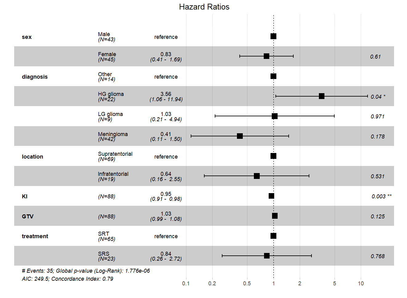
The forest plot in Figure 1 shows that in the variable Sex, Male category is the reference, and a hazard ratio is given for Female (0.83). The plot across shows the relative hazard with black square boxes. We can see that the hazard for Female is to the left of the dashed vertical line (denoting 1, no difference between two categories) and to the left of Male patients, implying that the hazard for Female category is lower than Male. In Diagnosis variable, the reference category is Other. We can see that HG Glioma is to the right of the reference (meaning higher hazard ratio), LG Glioma is almost aligned with the reference (close to 1 on the vertical dashed line), and Meninglomia is to the left of the reference, showing lower hazard. The variables KI and GTV are continuous predictors, therefore, there is no reference comparison, and only the position of the hazard relative to the vertical dashed line is shown. If the hazard is to the left of the dashed vertical line, it means the variable decreases the hazard.