STATISTICS with R
A comprehensive guide to statistical analysis in R
Chi-squared Test in R
The chi-squared test of independence is a statistical test that measures the relationship between categorical variables. For example, when we are interested in the relationship between two binary or categorical variables, we can use the chi-squared test of independence or association. The chi-squared test of independence is also known as the Pearson’s chi-squared test of independence or association.
Introduction to Chi-squared Test
When we are interested in the relationship between two binary or categorical variables, we can use the Pearson’s chi-squared test of association or independence.
A Pearson’s chi-squared test of association or independence measures the strength, direction, and significance of an association between two categorical variables, such as the association between smoking (smoker, nonsmoker) and heart problems (with heart problems, without heart problems), or the relationship between sex (male, female) and house ownership (own, not owned).
In a chi-squared test of association or independence, the term association is like a relationship but mostly used for describing the relationship between categorical variables. By independence, we mean we want to test if two categorical variables do not depend on each other (i.e., they have no relationship, and hence no dependence on each other).
The recorded data for the chi-squared test of association may come into two formats: raw count data and a summary count table. For example, suppose we are interested in knowing if there is an association between sleep position (with two values: sleeping on side, sleeping on back) and having backache (with two values: no backache, with backache). We randomly ask 55 patients if they have backache and what their sleep positions are before falling asleep. Each patient provides an answer to the backache question (with / without backache) and sleeping position question (sleeping on side, on back). We can populate these values in a table like Table 1 below.
| Patient | Sleep position | Back pain |
|---|---|---|
| Patient 1 | Side | No |
| Patient 2 | Side | Yes |
| Patient 3 | Back | No |
| Patient 4 | Back | Yes |
| Patient 5 | Side | Yes |
| … | … | … |
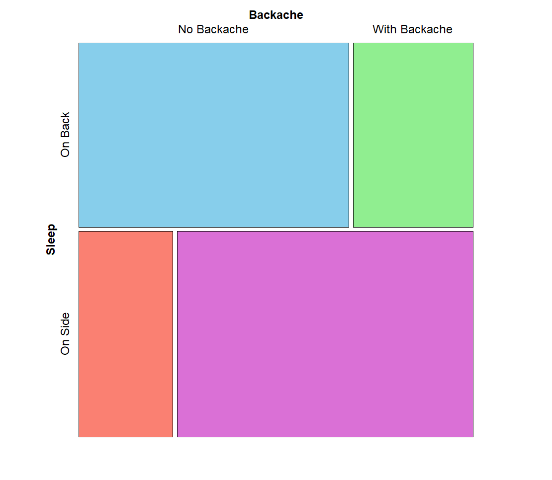
Another way to present data for the chi-squared test of association analysis is to use summary, contingency, or crosstab tables. Each contingency table has as many rows and columns as the number of levels or categories in each variable. For example, in the sleep position and backache data, we have two categories for sleep position (sleeping on side or on back) and two categories for backache (with or without backache). So, we have a 2 x 2 contingency or crosstab table. Each cell of the table includes the total number of co-occurrences of the levels of the variables. Table 2 demonstrates a contingency table for the sleep position and backache data.
| Sleep Position | Back Pain No | Back pain Yes |
|---|---|---|
| Back Sleepers | 18 | 8 |
| Side Sleepers | 7 | 22 |
Contingency tables, like Table 2 above, are usually read by row. For example, in Table 2, the row “Back sleepers” tells us that among those who sleep on their backs, 18 patients experienced no backache, and 8 patients did experience backache. In row “Side sleepers”, 7 patients didn’t experience backache, but 22 patients experienced backache. Apparently, Side sleepers had more backache complaints (22) compared to Back sleepers (7). So, is there a relationship between sleep position and backache complaints?
In the following sections, we demonstrate an example of a chi-squared test of association between two binary random variables and provide R code to quantify the strength, direction, and the statistical significance of the chi-squares test.
Chi-squared Test Example
Is there a relationship between Sleep position and having a Backache?

A public health researcher is interested in knowing if sleep position is associated with backache complaints among patients. The researcher randomly recruits 55 patients and asks them if they complained about backache and what sleep position they primarily had during the last year. Table 3 includes the responses to the two questions for five participants in the study.
| Student | Study Hours | Test Score |
|---|---|---|
| Student 1 | 31 | 70 |
| Student 2 | 32 | 75 |
| Student 3 | 44 | 100 |
| Student 4 | 32 | 80 |
| Student 5 | 28 | 83 |
| … |
The health researcher enters the data in a spreadsheet program in the computer and saves the data in the CSV format. The complete data set for this example can be downloaded from here.
Analysis: Chi-squared Test in R
In the first step, the researcher reads the data into the RStudio program using the read.csv() function. To conduct the chi-squared test of association between Sleep position and Backache complaint, we can use the chisq.test() function in base R. The chisq.test() is a built-in R function, and therefore, we do not need to install and load a package to use this function. The following code in Listing 1 shows how to perform a chi-squared test of association in R between two binary random variables.
# Read the data
dfSleep <- read.csv("dsSleepBackAche.csv")

# Crate the contingency table
cntgTable <- table(dfSleep$sleep_position, dfSleep$backache)

# Perform the chi-squared test on the contingency table
chsqTest <- chisq.test(cntgTable, correct = TRUE)

# Print the results of the chi-squared test
print(cntgTable)
print(chsqTest)


       Negative Positive
  Back       18        8
  Side        7       22


	Pearson's Chi-squared test with Yates' continuity correction

data:  cntgTable
X-squared = 9.498, df = 1, p-value = 0.002057The code in Listing 1 shows that after reading in the data and creating two variables for Sleep position and Backache complaint, we have performed the chi-squared test of association in two steps. In the first step, we have created a contingency table (cntgTable in the code) using the function table(). As explained above, a contingency table shows the sum of the counts of the two levels of the two variables. In the second step, we used the function chisq.test() on the contingency table we created to conduct the chi-squared test. The parameter correct = TRUE (Yates’ continuity correction) adjusts the chi-squared value (to reduce the likelihood of showing a false statistically significant result).
The output in Listing 1 shows the contingency table and the chi-squared test results. The contingency table shows the total number of cases in the joint level (co-occurrences) of the two variables. For example, the number of patients with Sleep position Back who didn’t have a backache is 18 and the number of Back sleepers with backache is 8. The number of Side sleepers who didn’t have backache is 7, and the number of side sleepers who complained of backache is 22. It seems there is an association. We look at the chi-squared results. Figure 1 shows a mosaic plot that visualizes the contingency table.
The chi-squared test results are shown under line Pearson’s Chi-squared test with Yates’ Continuity correction. The chi-squared value (shown as X-squared) is 9.498 with 1 degree of freedom and the p value is 0.002, which is statistically significant. So, we conclude that there is statistically significant association between Sleep position and having Back complaints.