STATISTICS with R
One-sample T-test in R
A one-sample t-test is a statistical method used to determine whether the mean of a single sample significantly differs from a known or hypothesized population mean. This test is particularly useful when researchers or analysts have a specific target or reference value and want to assess how a sample’s mean compares to that value. By evaluating the sample mean against the population mean, the one-sample t-test helps identify whether observed differences are likely due to random chance or if they indicate a statistically significant deviation.
Introduction to One-sample T-test
Commonly used in fields such as psychology, education, and medical research, the one-sample t-test provides a straightforward way to test hypotheses about population means, especially when dealing with small sample sizes and when the population standard deviation is unknown.
In certain studies, researchers aim to compare the mean score from a single sample to a standard or reference value. For instance, a health researcher might be interested in determining if the average blood pressure of a population has changed compared to the average blood pressure from several decades ago. The average blood pressure from that time serves as the reference value. The researcher randomly selects a sample from the current population, records their average blood pressure (and standard deviation), and seeks to determine if there has been an increase or decrease compared to the past population’s average blood pressure. The researcher does not have access to individual data from decades ago, only to the reference. However, individual data from the current population is available, allowing the calculation of both the mean and standard deviation. To assess whether the current average blood pressure significantly differs from the historical average, the researcher performs a one-sample t-test.
An important assumption when conducting a one-sample t-test is that the data should be normally distributed and the observations must be unrelated to each other.
In the following sections, we present an example research scenario where a one-sample t-test will be used to analyze the data. We will demonstrate how to perform a one-sample t-test in R step-by-step and how to interpret the results of one-sample t-test.
One-sample T-test Example
Is the average arsenic level in the school drinking water pipes within the limits of the EPA standard?

A high school science class aimed to determine if the drinking water quality in high schools within neighboring urban areas meets the Environmental Protection Agency (EPA) safety standards. Drinking water quality is assessed by measuring various organic and chemical compounds, including arsenic. According to the EPA, the acceptable level of arsenic in drinking water is 10 μg/L. The students randomly selected 32 high schools and collected water samples from the school building pipes on a school day. They then analyzed the water samples in their school laboratory to measure the arsenic levels. Table 1 displays the amount of arsenic found in the water from five schools.
| School | Arsenic Level in Water (μg/L) |
|---|---|
| School 1 | 6.29 |
| School 2 | 7.64 |
| School 3 | 5.98 |
| School 4 | 6.92 |
| School 5 | 8.09 |
| … | … |
The science class is interested in determining whether the mean arsenic level in the sampled water meets the EPA standard. If the sample mean is less than or equal to the standard, it is considered safe. If it is slightly higher, it may still be acceptable. However, if it is statistically significantly higher, it raises concern. One student enters the data in a spreadsheet program in the computer and saves the data in the CSV format. The complete data set for this example can be downloaded from here.
Analysis: One-sample T-test in R
In the first step, we create a CSV file to store the data. We create one column for the name of the school and another column for the level of arsenic. After reading in the data file into the RStudio program, we create a variable arsenicLevel from the data. Figure 1 shows the amount of arsenic in pipes in individual schools.
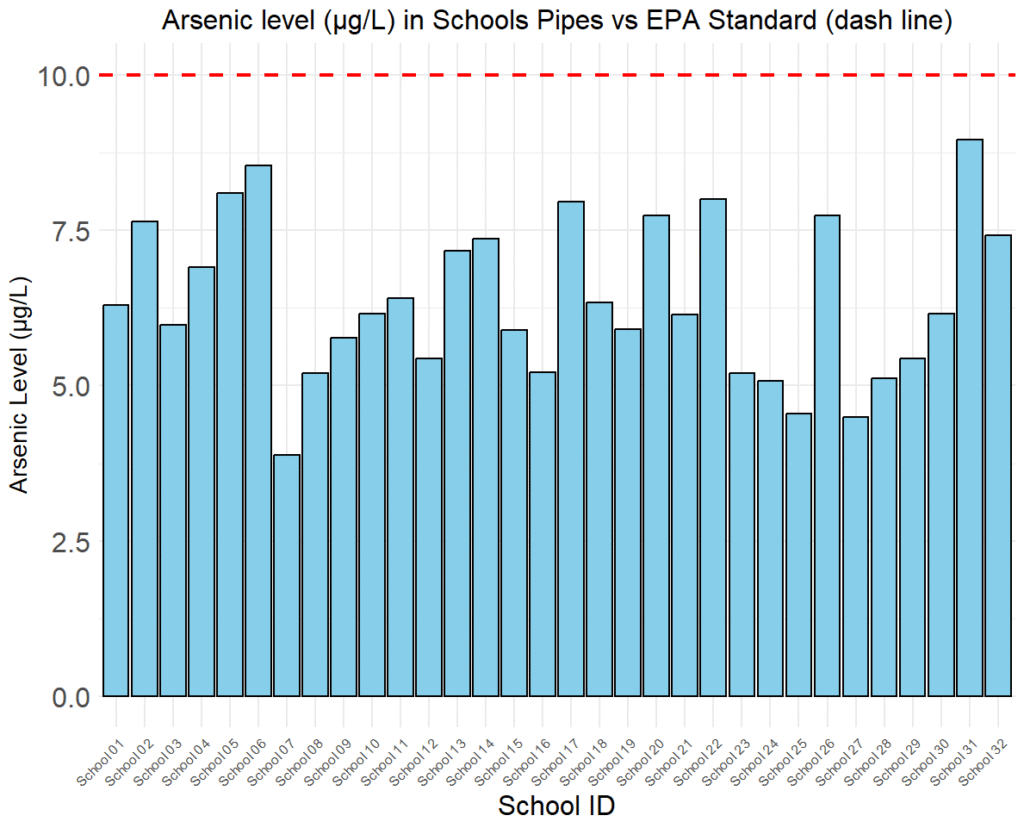
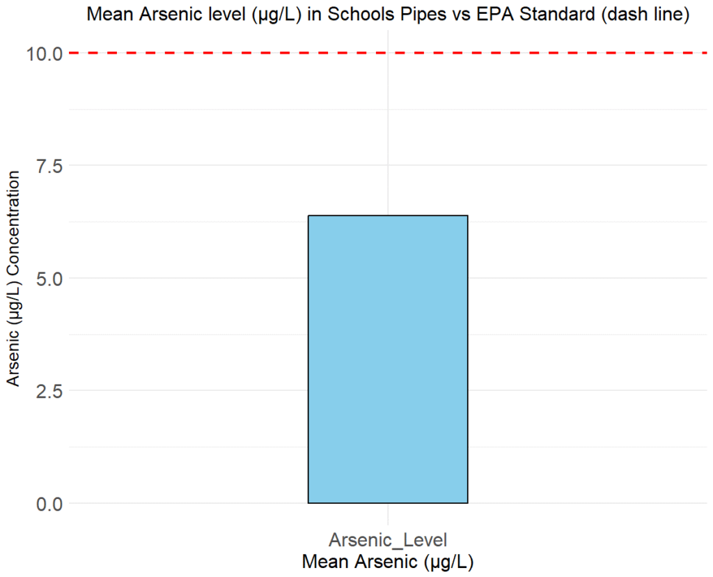
Figure 2 shows the amount of arsenic in pipes in individual schools. The red dashed line represents the EPA reference of 10 μg/L. The data points are below the EPA reference value, indicating that the arsenic level in the sampled waters is below the hazard threshold in individual schools. However, we are interested in knowing if the average arsenic level is statistically and significantly lower than the EPA reference. We perform a one-sample t-test to find out.
We perform a one sample t-test using the t.test function. The code is shown in Listing 1.
dfArsenic <- read.csv("dsArsenicLevel.csv")
arsenicLevel <- dfArsenic$Arsenic_Level
t.test(arsenicLevel, mu=10)

One Sample t-test

data: arsenicLevel
t = -15.968, df = 31, p-value < 2.2e-16
alternative hypothesis: true mean is not equal to 10
95 percent confidence interval:
5.916228 6.841272
sample estimates:
mean of x
6.37875The mean value for the arsenic level is 6.378 (μg/L), which is below the maximum threshold of 10 (μg/L) reference. (Figure 2).
The difference between the sample mean value and the reference mean is 3.621, which is statistically significant with observed t=-15.968, df=31, and p < 0.05. In addition, the 95% confidence interval for the mean arsenic level (5.916 to 6.841) does not include the EPA reference value of 10 μg/L, supporting rejection of the null hypothesis. Therefore, the science class can infer that the arsenic level in the collected samples is significantly below the reference maximum set by the health authorities.