STATISTICS with R
Simple Regression in R
Simple regression is a statistical method that measures and models the linear relationship between one independent variable and a continuous response variable. The independent variable (or predictor) can be continuous or discrete (categorical). Modelling means obtaining an equation from data that can be used to predict a future outcome. Regression is a fundamental method in predictive modeling.
Introduction to Simple Regression
The relationship between two random variables can be established using several measures of association and relationship, including Pearson correlation, Spearman correlation, and Kendall tau correlation. The correlation methods provide us with the strength and direction of a relationship summarized as a single number (correlation coefficient). These measures of association help us establish the existence or absence of a relationship. However, they stop there and cannot help us to predict a future value because they do not provide us with a prediction formula, equation, or a model.
Like physical phenomena (e.g., the time it takes a falling object to reach the ground surface), to predict a future value from a random variable, we need a model or equation. Regression takes correlation statistics to the modeling level by providing the researcher with an equation that establishes (models) the relationship between two random variables. In a linear relationship, regression analysis uses the line equation to establish the relationship between two variables. Therefore, similar to a line equation, a linear regression equation has an intercept (where the line crosses the y-axis) and a slope (the intercept-slope line equation). The slope of the line shows the relationship between the independent and the dependent variables: if the slope is large, the relationship is strong (and the other way round), and if the slope is negative, the relationship is inverse. The slope of the line is called the coefficient and denoted by the letter b1. The intercept is also shown by the letter b0. In a simple linear regression analysis, we are mostly interested in the coefficient (slope).
Linear regression analysis is a family of statistical methods that model the linear relationship between two random variables. The variable whose values we model and try to predict is called the dependent variable (usually shown by the letter “y”), and the variable that is used to predict those values of the dependent variable is called the independent variable (usually shown by the letter “x”). Other names for the dependent variables are the response, the outcome, or the target variable. Other names for the independent variable are the predictor, the explanatory, or the feature variable. In this chapter, we use the terms independent and dependent variables. Unlike correlation analysis, in a regression model we need to designate which variable is the dependent variable (y) and which variable is the independent variable (x).
A regression model is called a simple regression model if there is only one independent variable. If there are two or more than two independent variables, the regression is called a multiple regression model. The dependent variable in a simple or multiple regression is continuous (interval or ratio scale of measurement). However, the independent variables can be continuous, binary (two levels, like gender: male and female), or categorical (more than two levels, such as income: low income, middle income, and high income).
In the following sections, we introduce an example data set and demonstrate how to model the relationship between the independent and the dependent variable through a simple linear regression in R.
Simple Regression Example
What is the relationship between the number of hours that students study and their test scores? Can the number of study hours predict test scores?

A high school teacher is interested in modeling the relationship between the number of hours students study and the scores the students achieve on the test. The teacher randomly selects 65 students from the school district and asks the students how much time they dedicated to preparing for the test. The teacher is not only interested in understanding the relationship between study hours and test scores, but also if the number of studies can be used to predict a student’s test score. Table 1 includes the scores of five students on the test.
| Student | Study Hours | Test Score |
|---|---|---|
| Student 1 | 31 | 70 |
| Student 2 | 32 | 75 |
| Student 3 | 44 | 100 |
| Student 4 | 32 | 80 |
| Student 5 | 28 | 83 |
| … | … | … |
The teacher enters the data in a spreadsheet program in the school computer lab and saves the data in the CSV format. The complete data set for this example can be downloaded from here.
Analysis: Simple Regression in R
In the first step, data are read into the RStudio program using the read.csv() function. In this example, the dependent variable is the students’ test scores and the independent (predictor) variable is the number of study hours. Mathematically, we read such relationship as “test score is a function of study hours”, or “test score depends on study hours”. In mathematical notation, we write it as: test score ~ study hours. Similar mathematical formulation is used in R language to show the relationship between a dependent variable and an independent variable. The dependent variable is written on the left-hand side of the equation and the independent variable is written on the right-hand side of the equation.
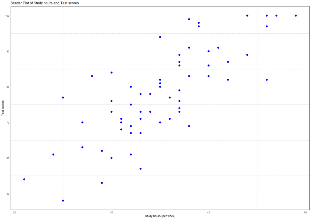
The teacher first plots the data in R to see if there is any apparent relationship, linearity, and any anomalies (e.g., extreme cases). Figure 1 shows a scatter plot of the relationship between study hours and test scores.
To perform a simple linear regression between the test scores and study hours, we use the lm() function in R. The lm() function is a built-in R function, and therefore, we do not need to install and call a package to use this function. We use the function notation (~) to show the relationship between the dependent variable (on the left-hand side) and the independent variable (on the right-hand side). The following R code in Listing 2 shows how to perform a simple linear regression between to model the relationship between two continuous random variables (study hours and test scores, in our example).
dfScores <- read.csv("dsStudyHoursTestScores.csv")

regStudyScores <- lm(testScore ~ studyHours, data = dfScores)
summary(regStudyScores)

# Output
Call:
lm(formula = testScore ~ studyHours, data = dfScores)

Residuals:
    Min      1Q  Median      3Q     Max
-17.349  -5.159  -0.266   4.247  17.164

Coefficients:
            Estimate Std. Error t value Pr(>|t|)
(Intercept)  18.1660     5.9435   3.056  0.00328 **
studyHours    1.7025     0.1667  10.216 5.41e-15 ***
---
Signif. codes:  0 ‘***’ 0.001 ‘**’ 0.01 ‘*’ 0.05 ‘.’ 0.1 ‘ ’ 1

Residual standard error: 8.073 on 63 degrees of freedom
Multiple R-squared:  0.6236,	Adjusted R-squared:  0.6176
F-statistic: 104.4 on 1 and 63 DF, p-value: 5.412e-15In this code, the parameters of the lm() function include the name of the dependent variable (test score), the name of the independent variable (study hours) and the name of the data set the two variables are in. The model and its parameters are given a name, regStudyScores (any arbitrary name). In this way, we create an object in the RStudio environment which carries several data and information bits, such as model formula and the results of the analysis. Therefore, we need another function to extract the desired information from the model object, such as summary(). This is the preferred way of building the model because later we may need to build another model and then compare the two models; hence we choose different names for our different models.
The simple linear regression results from the lm() function modeling the relationship between test scores and study hours outputs a fair amount of information. The Call line shows our formula model. Residuals show the difference between what our model predicts against the truth (i.e., actual data). Coefficients are the most important information we are interested in. The intercept is the point on the y-axis (dependent variable) where the line of best fits crosses (and where the x value, or the independent variable value is zero). In our example, the intercept is 18.166, meaning that when study hours is zero, we theoretically expect the test score to be 18.166. The next line in the Coefficients shows the coefficient for the independent variable “study hours”, which is 1.7025, and which is positive, and which is statistically significant.
The coefficient for the independent variable “study hours” is interpreted as follows: for each one hour of study, the test score increases on average 1.7025 scores. We say increases because the coefficient is positive. We can write the result of the analysis in terms of the relationship between the test score and study hours as following equation (model):
Expected test score = 18.166 + 1.7025*(study hours).
The equation above is our model and we can use it to predict a test score if we have information about the number of study hours. For example, if an individual studies for 25 hours a week, we predict their test score to be:
Expected test score = 18.166 + 1.7025*(25) = 60.728.
But is only one variable enough to predict a test score? This question can be answered by looking at the Adjusted R-squared value of 0.6176 in the last line of the results. R-squared represents the amount of variance (information) that can be explained by the independent variable in the model. In our example, we can say about 62% of the information we need to predict a test score is carried in the independent variable “study hours”. But we do not know what variables explain the rest of information (about 38% is unknown variance and/or error). Adjusted R-squared can be used as a measure of model adequacy (not model fit). It shows if we have enough information in our independent variable, or we need to replace or supplement it with other independent variables.